Filter Augmented JPEG Algorithms: A Critical Performance Study for Improving Bandwidth

(1)

Filter Augmented JPEG Algorithms: A Critical

Performance Study for Improving Bandwidth

Ch. Ramesh

Professor, Dept .of CSE AITAM, Tekkali, A.P, India

N.B. Venkateswarlu,

PhD.

Professor, Dept .of CSE AITAM, Tekkali, A.P, India

J.V.R. Murthy,

PhD.

Professor, Dept .of CSE College of Engineering,

JNTUK, A.P, India

ABSTRACT

In the recent years, use of Digital Image Communication has increased exponentially in the day to day activities. Joint Photographic Experts Group (JPEG) is the most widely used still image compression standard for bandwidth conservation. In this paper, it is proposed and critically studied a new set of JPEG Compression algorithms by combining Mean filtering, Median filtering, and Outlier detection algorithms and conventional JPEG DCT algorithm in a staged manner. This outlier based JPEG algorithm is giving exceptionally compression compared to conventional JPEG algorithm. Experiments are carried out with many standard still images. Algorithms developed in this paper, identified to be giving almost same Peak Signal-to-Noise Ratio (PSNR) as that of standard JPEG algorithm.

Key words:-

Mean, Median, Outlier, DCT, IDCT, PSNR, JPEG

1. INTRODUCTION

In the recent years, data intensive multimedia-based web applications have increased by many folds. Many remote applications such as remote monitoring, surveillance, automatic navigation systems often involves communication of captured images or videos for further processing. In these applications, it is inevitable to conserve the available bandwidth in order to reduce consumer side bills. In order to reduce the bills (or bandwidth consumption), communicating compressed images is a classical solution in communications and allied fields. In the literature, various algorithms were proposed for the image compression, and even many of them are available in embedded HW also. JPEG compression is the standard for image compression for still images. Its variants are under the name hood of MPEG (Motion Picture Experts Group) is widely followed standard for video encoding.

Image based recognition systems that are used in production industries such as IC manufacturing, fruit processing systems, automatic welding, etc., will be using original image. However, there are some recent applications such as remote monitoring, surveillance, remote surgery, etc., may involve communication of captured images to a server for processing, recognition and control. For example, [7] used compressed face images in JPEG format for the development of their face recognition system that extracts edge based features from the JPEG images and uses with a neural network. Certainly, performance of recognition system based on original images will be giving better results than compressed images as compressed images loses some details which are otherwise useful for recognition. It is reported elsewhere [12] JPEG

compression induces some artifacts such as noise around edges, blurring, a smeared appearance, color distortion, and/or checkerboard-like blocking in busy regions. However, it consumes very little bandwidth. Thus, scientific community

may be interested in studying about recognition system

performance when it is designed to use compressed images rather than original images. Authors [13] reports that JPEG images cannot be used for character recognition as JPEG distorts the sharp edges.

Herewith the authors propose a new set of image compression algorithms which uses Mean filtering, Median filtering, and Outlier detection concepts with conventional DCT algorithm in a staged manner that shows better edge images compared to conventional JPEG images. The average peak signal to noise ratio (PSNR) [1] of our algorithms is compared with original JPEG method.

The paper is organized as follows. In section 2, a brief overview of the JPEG standard is provided. The proposed Mean, Median & Outlier based JPEG compression system is described in section 3. Experimental results are presented in section 4. Finally, conclusions are reported in section 5.

2. BRIEF OVERVIEW OF JPEG

ENCODING / DECODING SYSTEM

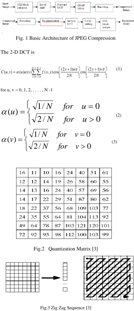
JPEG is a well known standardized image compression technique. JPEG loses information so the decompressed picture is not the same as the original one. The main reason for use of JPEG is to reduce the size of image files. Reducing image files is an important procedure for transmitting files across networks or archiving libraries. Usually JPEG can remove the less important data before the compression; hence JPEG is able to compress images meaningfully, which produces a huge difference in the transmission time and the disk space. Fig 1 shows the basic Architecture of JPEG compression system. Here is a brief overview of the JPEG compression system. [2]

The image is first subdivided into pixel blocks of size 8X8, which are processed left to right and top to bottom. As each 8X8 block or sub image is encountered, its 64 pixels are level shifted by subtracting the quantity L/2, where L is the Gray level resolution of the image. The 2-D Forward Discrete Cosine Transform (FDCT) (Eq 1) [5] of the block is then computed, quantized using 64 corresponding step size values

from the quantizationtable in Fig.2[3]. After quantization the

(2)

Since the one-dimensional reordered array generated under the zigzag pattern of Fig.3 is qualitatively arranged according to increasing spatial frequency, the JPEG coding procedure is designed to take the advantage of the long runs of zeros that normally result from the reordering. In particular, the nonzero AC coefficients (the term AC denotes all transform

coefficients with the exception of the zeroth or DC coefficient)

[image:2.595.53.285.203.739.2]

are coded using a variable-length code that defines the coefficient’s value and number of preceding zeros. The DC coefficient is difference coded relative to the DC coefficient of the previous sub image.

Fig. 1 Basic Architecture of JPEG Compression

The 2-D DCT is



               1 0 1 0 2 ) 1 2 ( cos 2 ) 1 2 ( cos ) , ( ) ( ) ( ) , ( N x N y N v y N u x y x f v u v u

C     (1)

for u, v = 0, 1, 2, . . . . , N -1











0 /

2

0 /

1 )

(

u

for

N

u

for

N

u



₍₂₎











0 /

2

0 /

1 )

(

v

for

N

v

for

N

v



(3)

Fig.2 Quantization Matrix [3]

Fig.3 Zig Zag Sequence [3]

The decompression process performs an inverse procedure. It

the Quantization step. In this stage, the decoder raises the small numbers by multiplying them by the quantization coefficients. The results are not accurate, but they are close to the original numbers of the DCT coefficients. An Inverse Discrete Cosine Transform (IDCT) (Eq.4) [6] is performed on the data received from the previous step. Finally add L/2 to each sub image. Place the sub images in their correct positions.



               1 0 1 0 2 ) 1 2 ( cos 2 ) 1 2 ( cos ) , ( ) ( ) ( ) , ( ˆ N u N v N v y N u x v u C v u y x

f





(4)

The error between the original image and reconstructed image

is calculated in terms of Peak signal to noise ratio

(PSNR) = 10 log10 (L

2

/MSE) (5)





mXn

y

x

f

y

x

f

MSE

m x n y



   





1 0 1 0 2

)

,

(

)

,

(

ˆ

(6)

MSE – Mean Squared Error

)

,

(

ˆ

_x

_y

f

- Reconstructed Image

f (x, y) – Original Image m x n – Size of the Image

3. NEW MEAN, MEDIAN & OUTLIER

BASED JPEG ALGORITHMS

Mean filtering [8] is a simple, intuitive and easy to implement method of image smoothing i.e. reducing the amount of variation between one pixel and the next or surrounding pixels. It is often used to reduce noise in image. The idea of mean filtering is simply to replace each pixel in an image with the mean value of its neighbors including itself. This has the effect of eliminating pixel values which are unrepresentative of their surroundings. Usually, 3x3 neighborhoods of pixels are considered while calculating mean filtered value of any pixel.

Median filter [9] is normally used to reduce noise in an image like the mean filter. However, it often does a better job than the mean filter in preserving useful detail in the image. Like the mean filter, the median filter considers each pixel in the image in turn and looks at its neighbors to decide whether or not its representative of its surroundings. Instead of simply replacing the pixel value with the mean of neighboring pixel values, it replaces it with the median of those values.

An outlier [11] is an observation that is numerically distant from the rest of the data. In an image, a pixel value is very different from its surrounding pixels, it can be called as outlier. Certainly, replacing its value with mean filtered or median filtered or DCT based with induce noise into our image. Thus, the authors propose to retain its value as it is such that noise will become less and more over subsequent edge detection results will be attractive for image recognition

systems.

(3)

Critical Values [10]. In the outlier based algorithms, take this simple confidence limits of normal distribution in deciding whether a pixel is outlier or not. If the pixel is observed to be outlier with the given confidence level, one may retain else may take its mean filtered or median filtered value.

Confidence Level 80% 90% 95% 98% 99% 99.80% 99.90% Critical Values 1.28 1.645 1.96 2.33 2.58 3.08 3.27

In the following, the authors listed the basic Mean, Median and outlier algorithms

3.1 MeanDCT Algorithm

1. Apply mean filtering to the original image using 3x3

window

2. Apply DCT on the mean filtered images

3.2 MedianDCT Algorithm.

1. Apply median filtering to the original image using 3x3

window

2. Apply DCT on the mean filtered images

3.3 Outlier MeanDCT Algorithm

1. Apply mean filtering with a little variation to the given

original image using 3x3 window. For each pixel, calculate average and standard deviation of its neighboring 3x3 pixels. If a pixels value is observed to be outlier (not in the range of Mean ± C*σ) then its filtered value is taken as itself else mean is taken as its filtered value.

2. Apply DCT on the mean filtered image.

3.4 Outlier MedianDCT Algorithm

1 Apply median filtering with a little variation to the given

original image using 3x3 window. For each pixel, calculate average and standard deviation of its neighboring 3x3 pixels. If a pixels value is observed to be outlier (not in the range of Mean ± C*σ) then its filtered value is taken as itself else median is taken as its filtered value.

2 Apply DCT on the median filtered image.

4. EXPERIMENTAL WORK

In this study, the authors have used a number of images in tiff

format from USC-SIPI image database

“http://sipi.usc.edu/database” [4]. Experiments are carried out

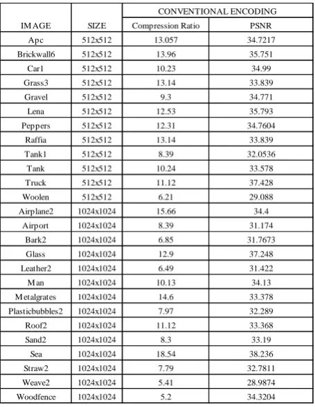
[image:3.595.316.544.100.394.2]

under MS Windows XP version 2002, SP3 edition. The experimental system is equipped with Intel core 2 Duo 2.60 GHz processor with 1 GB RAM. Programs are written in C language under Microsoft Visual Studio 2005 version 8.0. Table 2 illustrates conventional JPEG compression ratios and PSNR values of the selected images [4]

Table 2: Compression ratios and PSNR values of the selected images with conventional JPEG.

Compression Ratio PSNR

Apc 512x512 13.057 34.7217

Brickwall6 512x512 13.96 35.751

Car1 512x512 10.23 34.99

Grass3 512x512 13.14 33.839

Gravel 512x512 9.3 34.771

Lena 512x512 12.53 35.793

Peppers 512x512 12.31 34.7604

Raffia 512x512 13.14 33.839

Tank1 512x512 8.39 32.0536

Tank 512x512 10.24 33.578

Truck 512x512 11.12 37.428

Woolen 512x512 6.21 29.088

Airplane2 1024x1024 15.66 34.4

Airport 1024x1024 8.39 31.174

Bark2 1024x1024 6.85 31.7673

Glass 1024x1024 12.9 37.248

Leather2 1024x1024 6.49 31.422

M an 1024x1024 10.13 34.13

M etalgrates 1024x1024 14.6 33.378

Plasticbubbles2 1024x1024 7.97 32.289

Roof2 1024x1024 11.12 33.368

Sand2 1024x1024 8.3 33.19

Sea 1024x1024 18.54 38.236

Straw2 1024x1024 7.79 32.7811

Weave2 1024x1024 5.41 28.9874

Woodfence 1024x1024 5.2 34.3204

IM AGE SIZE

CONVENTIONAL ENCODING

(4)

[image:4.595.54.290.84.661.2]

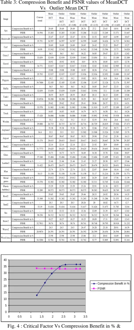
Table 3: Compression Benefit and PSNR values of MeanDCT Vs Outlier Mean DCT

M ean Outlier Outlier Outlier Outlier Outlier Outlier Outlier DCT M ean M ean M ean M ean M ean M ean M ean

DCT (C=3.27) DCT (C=3.08) DCT (C=2.58) DCT (C=2.33) DCT (C=1.96) DCT (C=1.645) DCT (C=1.28) Compression Benefit in % - 29.49 29.49 29.49 28.74 27.2 23.63 18.91 11.88

PSNR 34.594 33.203 33.203 33.203 33.206 33.222 33.269 33.371 33.647 Compression Benefit in % - 22.47 22.47 22.47 22.54 21.52 18.87 14.99 10.67 PSNR 35.751 34.597 34.597 34.597 34.599 34.605 34.626 34.723 34.961 Compression Benefit in % - 24.69 24.69 24.69 24.65 24.42 23.22 20.47 15.27 PSNR 34.99 33.542 33.542 33.542 34.543 33.548 33.596 33.73 34.024 Compression Benefit in % - 36.5 36.5 36.5 36.22 34.85 29.47 22.33 12.82 PSNR 33.839 32.939 32.939 32.939 33.043 33.054 33.1 33.189 33.389 Compression Benefit in % - 18.92 18.92 18.92 18.9 18.76 18.05 16.53 12.78 PSNR 34.771 32.817 32.817 32.817 33.818 32.82 32.842 32.905 33.142 Compression Benefit in % - 19.08 19.08 19.08 18.95 18.56 17.61 15.71 12.15 PSNR 35.793 32.937 32.937 32.937 33.936 32.936 32.952 33.009 33.347 Compression Benefit in % - 19.2 19.2 19.2 19.02 18.51 16.8 14.4 11.06 PSNR 34.7604 32.105 32.105 32.105 32.106 32.197 32.126 32.176 32.307 Compression Benefit in % - 36.5 36.5 36.5 36.22 34.85 29.47 22.33 12.82 PSNR 32.839 33.039 33.039 33.039 33.043 33.954 33.1 33.189 33.389 Compression Benefit in % - 28.55 28.55 28.55 28.45 28.12 26.13 22.05 15.06 PSNR 32.0536 30.288 30.288 30.288 30.29 30.3 30.367 30.52 30.873 Compression Benefit in % - 29.62 29.62 29.62 29.41 28.86 26.37 22.31 14.51 PSNR 33.578 31.903 31.903 31.903 31.906 31.919 31.977 32.109 32.457 Compression Benefit in % - 16.83 16.83 16.83 16.79 16.73 16.58 16.1 14.26 PSNR 37.428 36.886 36.886 36.886 35.888 35.892 35.902 35.938 36.081 Compression Benefit in % - 33.2 33.2 33.2 33.13 32.55 29.8 24.6 16.42 PSNR 29.088 26.715 26.715 26.715 26.716 26.729 26.819 27.026 27.473 Compression Benefit in % - 35.38 35.38 35.38 34.73 32.86 27.62 20.73 11.77 PSNR 34.4 33.5 33.5 33.5 33.502 33.508 33.524 33.585 33.79 Compression Benefit in % - 30.67 30.67 30.67 30.53 29.98 27.63 23.38 16.13 PSNR 31.174 28.615 28.615 28.615 28.617 28.623 28.667 28.799 29.207 Compression Benefit in % - 22.14 22.14 22.14 22.11 21.92 20.9 18.69 14.42 PSNR 31.7773 29.625 29.625 29.625 29.625 29.634 29.693 29.841 30.185 Compression Benefit in % - 34.73 34.73 34.73 34.69 34.38 33.78 32.84 30.07 PSNR 37.248 33.404 33.404 33.404 33.404 33.404 33.409 33.421 33.498 Compression Benefit in % - 21.46 21.46 21.46 21.43 21.27 20.38 18.57 15.66 PSNR 31.422 28.473 28.473 28.473 28.473 28.478 28.523 28.651 29.016 Compression Benefit in % - 22.74 22.74 22.74 22.52 22.07 20.69 18.16 13.62 PSNR 34.13 31.158 31.158 31.158 31.158 31.17 31.214 31.359 31.771 Compression Benefit in % - 25.012 25.012 25.012 24.92 24.29 22.65 17.56 11.39 PSNR 33.378 32.302 32.302 32.302 32.302 32.311 32.765 32.424 32.644 Compression Benefit in % - 23.29 23.29 23.29 23.24 22.91 21.36 18.53 13.57 PSNR 32.289 30.573 30.573 30.573 30.575 30.583 30.635 30.749 31.035 Compression Benefit in % - 29.65 29.65 29.65 29.46 28.53 24.92 20.36 14.35 PSNR 33.368 31.262 31.262 31.262 31.263 31.268 31.286 31.353 31.62 Compression Benefit in % - 20.3 20.3 20.3 20.26 20 18.82 16.73 12.7 PSNR 33.19 31.616 31.616 31.616 31.617 31.626 31.673 31.783 32.04 Compression Benefit in % - 22.32 22.32 22.32 22.26 22.09 21.29 18.27 12.82 PSNR 38.236 36.312 36.312 36.312 36.312 36.312 36.319 36.344 36.46 Compression Benefit in % - 18.27 18.27 18.27 18.25 18.09 17.31 15.65 12.43 PSNR 32.7811 30.74 30.74 30.74 30.741 30.748 30.795 30.918 31.232 Compression Benefit in % - 24.5 24.5 24.5 24.47 24.28 23.18 20.91 16.39 PSNR 28.9874 26.391 26.391 26.391 26.392 26.399 26.454 26.594 26.061 Compression Benefit in % - 23.98 23.98 23.98 23.86 23.2 20.61 16.69 10.84 PSNR 34.3204 32.761 32.761 32.761 32.762 32.77 32.805 32.891 33.161 Sand2 Sea Straw2 Weave2 Wood fence Roof2 Tank Truck Woolen Airplane2 Airport Bark2 Glass Leather2 M an M etal grates Plastic bubbles2 Tank1 Image Conven tional Apc Brickwall6 Car1 Grass3 Gravel Lena Peppers Raffia

Fig. 4 : Critical Factor Vs Compression Benefit in % & Critical Factor Vs PSNR for Image “Gravel” with

OutlierMeanDCT

Figure 4 shows As the C value increases, Compression Benefit increases and PSNR decreases. The variation in PSNR is very small as the C value increases. The PSNR values are very nearer to the PSNR values obtained by conventional JPEG coding.

Table 4 shows the Compression Benefit and PSNR values of MedianDCT algorithm Vs OutlierMedianDCT algorithm.

With all the images it is found that MedianDCT and

[image:4.595.315.536.242.705.2]

OutlierMedianDCT algorithms have better compression ratios as compared to conventional JPEG coding. The PSNR loss in MedianDCT and OutlierMedianDCT algorithms is negligible as compared to conventional JPEG coding. While comparing MedianDCT and the corresponding Outlier DCT, Compression Benefit in %s are observed to be MedianDCT>OutlierMedianDCT(for C=1.28 to 2.58). As the value of C increases in the Outlier, Compression Benefit increases. For C=3.08 to 3.27 Compression Benefit in MedianDCT and OutlierMedianDCT is same. PSNR in MedianDCT<OutlierMedianDCT(for C=1.28 to 2.58). As the value of C decreases in the Outlier, PSNR increases. For C=3.08 to 3.27 PSNR in MedianDCT and OutlierMedianDCT is Same.

Table 4 Compression Benefit and PSNR values of MedianDCT Vs OutlierMedianDCT

Outlier Outlier Outlier Outlier Outlier Outlier Outlier M edian M edian M edian M edian M edian M edian M edian

DCT (C=3.27) DCT (C=3.08) DCT (C=2.58) DCT (C=2.33) DCT (C=1.96) DCT (C=1.645 DCT (C=1.28) Compression

Benefit in % - 27.58 27.58 27.58 26.9 25,57 22.14 17.58 10.65 PSNR 34.594 32.29 32.29 32.29 30.304 33.342 33.468 33.66 34.04 Compression

Benefit in % - 17.34 17.34 17.34 16.79 16.37 14.4 11.41 7.22 PSNR 35.751 35.043 35.043 35.043 35.044 35.058 35.105 35.206 35.405 Compression

Benefit in % - 13.21 13.21 13.21 13.15 12.89 12 10.45 7.26 PSNR 35.793 34.034 34.034 34.034 34.034 34.042 34.082 34.197 34.876 Compression

Benefit in % - 24.4 24.4 24.4 24,29 23.91 22.05 18.22 11.67 PSNR 32.0536 30.405 30.405 30.405 30.41 30.428 30.522 30.73 31.162 Compression

Benefit in % - 18.08 18.08 18.08 18.06 17.92 17.01 15.1 11.26 PSNR 28.9874 26.841 26.841 26.841 26,842 26.854 26.93 27.101 27.489 Compression

Benefit in % - 20.43 20.43 20.43 20.03 19.5 17.4 13.89 8.31 PSNR 34.3204 33.518 33.518 33.518 33.245 33.346 33.318 33.439 33.853 Wood fence Bark2 Glass Leather2 M an M etalgrates Plastic bubbles2 Roof2 Sand2 Sea Straw2 Weave2 Airport Car1 Grass3 Gravel Lena Peppers Raffia Tank1 Tank Truck Woolen Airplane2 Brickwall6

Image Conven _tional M edianDC T Apc 0 5 10 15 20 25 30 35 40

0 0.5 1 1.5 2 2.5 3 3.5

(5)

[image:5.595.55.285.71.182.2]

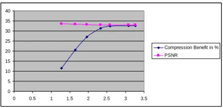
Fig. 5 : Critical Factor Vs Compression Benefit in % & Critical Factor Vs PSNR for Image “Gravel” with

OutlierMedianDCT

Figure 5 shows As the C value increases, Compression Benefit increases and PSNR decreases. The variation in PSNR is very small as the C value increases. The PSNR values are very nearer to the PSNR values obtained by conventional JPEG coding.

In a nutshell, the experiments indicated the following,

1. Compression Benefit of algorithms are observed to be

MeanDCT>MedianDCT> ConventionalDCT

2. PSNR of algorithms are observed to be

MeanDCT<MedianDCT <ConventionalDCT

3. While comparing MeanDCT and the corresponding

OutlierDCT, Compression Benefit are observed to be MeanDCT>OutlierMeanDCT (for C=1.28 to 2.58). As the value of C decreases in the Outlier, Compression Benefit decreases.For C=3.08 to 3.27 Compression Benefit in MeanDCT and OutlierMeanDCT is same.

4. While comparing MeanDCT and the corresponding

OutlierDCT, PSNR is observed to be Mean-DCT<OutlierMeanDCT. (for C=1.28 to 2.56) As the value of C decreases in the Outlier, PSNR increases. For

C=3.08 to 3.27 PSNR in MeanDCT and

OutlierMeanDCT is same.

5. While comparing MedianDCT and the corresponding

OutlierDCT, Compression Benefit are observed to be MedianDCT>OutlierMedianDCT (for C=1.28 to 2.58). As the value of C decreases in the Outlier, Compression Benefit decreases. For C=3.08 to 3.27 Compression Benefit in MedianDCT and OutlierMedianDCT is same.

6. While comparing MedianDCT and the corresponding

OutlierDCT, PSNR is observed to be Median-DCT<OutlierMedianDCT (for C=1.28 to 2.56) as the value of C decreases in the Outlier, PSNR increases. For

C=3.08 to 3.27 PSNR in MedianDCT and

OutlierMedianDCT is same.

7. All the retrieved images based on Conventional JPEG

system and Mean, Median & Outlier based JPEG system are almost same for visual appearance.

8. All the error images based on Conventional JPEG system

and Mean ,Median & Outlier based JPEG system are negligible

In the recent years, value added multi-media services are gaining importance. Here, the consumer will be billed in accordance with the quality of service he has enjoyed. All of the algorithms are best suitable at this junction as they have freedom to control the quality with decreasing C.

5. CONCLUSIONS

In this paper, new MeanDCT, MedianDCT,

OutlierMeanDCT & OutlierMedianDCT based JPEG

compression algorithms are proposed. The authors have compared these MeanDCT, MedianDCT, OutlierMeanDCT & OutlierMedianDCT based JPEG compression algorithms with Conventional JPEG compression. From these experiments it is evident that these approaches gives better compression ratios compared to conventional JPEG. The PSNR resulting from the approach is slightly less than Conventional approach. The PSNR resulting from OutlierMedianDCT with lowest critical factor is almost same as conventional approach. Highest Compression Benefit is achieved from OutlierMeanDCT with highest critical factor. However, all the decoded images resulting from this approach and original images are almost the same in human perception point of view.

6. REFERENCES

[1] Muhammad F.Sabir, Hamid Rahim Sheikh, Robert W.Heath, Alan C.Bovik” A Joint Source-Channel Distortion Model for JPEG Compressed Images” IEEE Transictions on Image Processing Vol 15, No 6, pp1349-1364 June 2006

[2] Cung Nguyen “Detecting Computer –Induced Errors in Remote-Sensing JPEG Compression Algorithms” IEEE Transictions on Im age Processing Vol 15, No 7, pp1728-1739 July 2006

[3] R.C.Gonzalez and R.E.Woods “Digital Image

Processing”, 2nd Edition Addison Wesley, USA ISBN: 0-201-60078, 1993sz

[4] The USC–SIPI image database

(http://sipi.usc.edu/database). Signal and image

processing institute Ming Hgieh Department of Electrical Engineering.

[5] Andrew B.Watson “Image Compression using the discrete cosine transform” Mathematica Journal 4 (1), 1994, p-81-88

[6] Ken cabeen and peter gent,” Image compression and the discrete cosine transform”, Math 45 college of redwoods

[7] K. Kantapanit and W. Wiriyasuttiwong. “Face

Recognition by Edge Detection of JPEG Compressed Images and Backpropagation Neural Network” The Engineering Journal of Siam University. Volume 3, Year 2 , July-December, 2000.

[8] “Mean filtering, Smoothing, Averaging, Box

filtering”,http://homepages.inf.ed.ac.uk/rbf/HIPR2/mean. htm

[9] “Median filtering, Rank filtering” http://homepages.inf. ed.ac.uk /rbf /HIPR2/median.htm

[10] “Cofidence Intervals”,http://www.stat.yale.edu/

courses/1997-98/101/confint.htm

[11] “Working with outliers”, http://en.wikipedia.org/ wiki/ outlier

[12] “JPEG Artifacts “,http://graphicssoft.about.com/od/

glossary/ g/jpegartifacts.htm

[13] “JPEG Artifacts”, http://www.scantips.com/

basics9jb.html

0 5 10 15 20 25 30 35 40

0 0.5 1 1.5 2 2.5 3 3.5