The DNA ejection process in bacteriophage lambda

(1)

The DNA ejection process in bacteriophage

λ

Thesis by

Paul Grayson

In Partial Fulfillment of the Requirements

for the Degree of

Doctor of Philosophy

California Institute of Technology

Pasadena, California

2007

(2)

Abstract

Bacteriophages have long served as model systems through which the nature of life may be explored. From

a physical or mechanical point of view, phages are excellent examples of natural nanotechnology: they

are nanometer-scale systems which depend critically on forces, pressures, velocities, and other

fundamen-tally physical quantities for their biological functions. The study of the physical properties of phages has

therefore provided an arena for application of physics to biology. In particular, recent studies of the motor

responsible for packaging a phage gnome into a capsid showed a buildup of pressure within the capsid of

tens of atmospheres. This thesis reports a combined theoretical and experimental study on various aspects of

the genome ejection process, so that a comparison may be drawn with the packaging experiments. In

partic-ular, we examine various theoretical models of the forces within a phage capsid, deriving formulas both for

the force driving genome ejection and for the velocity at which the genome is translocated into a host cell.

We describe an experiment in which the force was measured as a function of the amount of genome within

the phage capsid, and another where the genome ejection velocity was measured for single phages under

the microscope. We make direct quantitative comparisons between the theory and experiments, stringently

(3)

Introduction

1.1 Phages as an arena for science

For the past fifty years, bacteriophages have served as excellent systems for studying the physics of

biolog-ical molecules at the nanometer scale, capable tools for biotechnology, and basic examples through which

we can better understand the processes of life. The reason that phages have been so widely used in the

bio-logical sciences is that they are some of nature’s simplest machines, consisting of little more then a tightly

coiled piece of genetic material enclosed by a strong protein shell, thecapsid. Phages can be easily

puri-fied whole or as separate components, and every phase of the lifecycle can be isolated and studiedin vitro.

Studying these simple machines can reveal properties of DNA, RNA, and proteins, teaching us how they

work together to allow the phage to reproduce.

1.1.1 The central position of phages in biology

Phages occupy a central position in the history of biology and continue to serve important roles throughout

the life sciences. Their simple life cycle, small size, and the ease with which wild phages may be tamed in

the laboratory makes them ideal units for performing many kinds of experimental manipulations, and their

huge diversity makes them readily available for many applications: the number of phages and phage species

exceed those of the bacteria by about an order of magnitude (Fuhrman 1999; Rohwer 2003). Here we will

list a few of the areas in which phages have had and continue to have a tremendous impact on biology.

In 1943, Luria and Delbr¨uck conducted an experiment using phageαthat was a quantitative

demonstra-tion that mutademonstra-tions occur randomly rather than in response to a selecdemonstra-tion event. By counting the numbers

(8)

the mutations occurred before the bacteria were exposed to phages. This experiment, together with a

simi-lar demonstration using phage T1 (Newcombe 1949), cemented the idea that random mutation is followed

by natural selection. It is interesting that the results of the experiments make sense only in the context of

specific mathematical models: this quantitative approach is reflected in the organization of this thesis.

McCarty and Avery used purified bacterial DNA to show that DNA is the material responsible for

car-rying genetic information. However, the scientific community was not convinced by this result until later,

when phages provided Hershey and Chase (1952) with a conceptually simple system for distinguishing

be-tween DNA and protein. Interestingly, the experiment of Hershey and Chase took place right around the

same time as the discovery of the structure of DNA (Watson and Crick 1953; Franklin and Gosling 1953).

It worked as follows: phage T2 was labeled either with radioactive32P or35S, targeting the DNA or the

protein, respectively. Then the phages were mixed with host E. colicells, into which the genetic

mate-rial was injected. The experimenters sheared the phage-cell complexes in a blender, separating the capsids

permanently from the injected genetic material. Genetic material remained in the cells, which could be

re-moved from solution by centrifugation, while the phage capsids remained suspended. Comparing sediment

to supernatant, it was shown that the genetic material contained32P, proving that it was made of DNA. The

claim that the genetic material is injected DNA clearly holds true to this day, though some exceptional cases

have been found among the phages, such as phage N4, which injects protein along with its DNA (Davydova

et al.2003). Further contributions to our understanding of the gene came from phage-based studies of the

genetic code, such as the map of the fine structure of a region of the phage T4 genome by Benzer (1955) or

R. Feynman’s unpublished study of frame-shift mutations in the same bacteriophage (Cricket al.1961).

Phages can function as tools for genetic engineering. Soon after the determination of the structure of

DNA, it was shown that phages could exchange entire genes between strains of bacteria through

trans-duction, a technique that is still in common use today Morseet al.(1956). With the discovery of

restric-tion enzymes, it became possible to constructvectors by directly cutting and splice genes of interest into

phages (Murray and Murray 1974; Rambach and Tiollais 1974; Thomaset al.1974; Tiollaiset al.1976).

At the cost of some added complexity, phages have technical advantages as vectors. For example, the phage

DNA packaging and ejection system is a more efficient method for transferring DNA into cells. For

ex-ample, the Lambda ZAP II system (Stratagene) allows up to a 10 kbp insert, with an efficiency of 1/2000,

(9)

technique ofphage display, in which a protein of interest is expressed on the phage capsid, allows anin vitro

connection to be made between gene and function. For example, a particular binding affinity can be tested,

and the genes producing high-affinity proteins can be recovered directly from the substrate (Dufneret al.

2006).

In the environment, phages constantly swap genes between distantly related species of bacteria, in an

example of what is known ashorizontal gene transfer. Horizontal gene transfer clouds our understanding of

evolution. For example, the gene encoding the 16S ribosomal RNA is commonly used as a marker to study

the position of cells on the tree of life. Suppose speciesAhas a similar 16S gene to that ofE. coli. Then we

would place it on a branch of the tree close toE. coli, indicating a close relationship. However, if the 16S

gene was transferred toA106_{years ago via a phage, the rest of the genes of}_A_{could be totally unrelated. In}

fact, it is expected that this process has occurred very often throughout evolutionary history, making it much

more difficult to trace genes backwards and learn about the origin of life (Hommaet al.2007).

Phage-mediated gene transfer in the environment also has critical relevance for human health. Some

of the genes commonly transferred by phages induce pathogenicity in bacteria: for example, the toxin that

causes the diseaseCholerais produced by a gene that must be transferred to the cell via a bacteriophage

(Pol-litzer 1955; O’Shea and Boyd 2002). In fact, given the potential for virus-mediated gene exchange between

species, it is not surprising that similarities have been found between phages and plant, human, and archaeal

viruses. The principles we will learn by studying phages can apply to all domains of life (Riceet al.2004;

Hendrix 2004).

1.1.2 Phages as a focus of physical research in biology

Phages have also long been the focus of attention of physicists studying biology. As simple biological

machines with a well-defined, geometric structure, phages allow quantitative studies of biology, giving us

hope that a part of life can be completely understood via physical models. Different kinds of physical

models apply to different stages of the phage lifecycle, beginning with the gene regulation that produces

phage proteins and copies the genome in the correct quantity and at the correct time, followed by capsid

assembly and genome packaging, lysis of the host cell, receptor binding, and ejection of the genome into a

new host.

Since phages have few genes, their regulation is relatively simple, but each phage has unique features

(10)

pathways inλ, which was discussed in detail by Ptashne (1992). The protein CI maintains the lysogenic

state but also represses its own production via a process that involves folding 2.4 kbp of DNA into a loop.

This loop allows a long-range cooperativity that is crucial to turning on repression at the right concentration

of CI. Single-molecule quantitative studies are currently leading the way in understanding the dynamics of

loop formation that is critical to the genetic regulation ofλ(Zurlaet al.2006).

For a phage to reproduce, it must assemble new capsids from identical proteins, presenting a challenging

modeling problem: how do many identical copies of an protein “know” how to form a large capsid of precise

dimensions? The geometric complexity of an icosahedral phage capsid is characterized by what is known

as theT number. A minimal icosahedral phage has 60 copies of its capsid protein, three for each face of

the icosahedron, and is labeled asT = 1. More complex phages can be formed by replacing each triangle with some numberT of triangles. For example,λis aT = 7bacteriophage (Dokland and Murialdo 1993), which means it has approximately7×60 = 420copies of its capsid proteins gpE and gpD. Some of the proteins must arrange themselves into groups of 6-fold symmetry, while there must be exactly 12 groups of

5-fold symmetry for the icosahedron to form. It is interesting that the proteins always form the right ratio

of 5-fold to 6-fold groups and that they succeed in making a shell of consistentT number. Various models

seek to explain the assembly in terms of both equilibrium (Zandiet al.2004) and non-equilibrium (Hicks

and Henley 2006) descriptions.

Once a phage capsid is assembled, an energy-consuming motor packs DNA into the capsid, raising the

questions of how the DNA is arranged and how much force is required to force it entirely inside.

Earn-shaw and Harrison (1977) used X-ray scattering to determine thatλDNA is packed to a density of about

500 mg/mL, so that it takes up 50% of the volume of the capsid. Later, Cerritelliet al.(1997) recorded

cry-oelectron micrographs of phage T7 clearly showing circular loops of DNA packed into a hexagonal lattice.

It is thought that the DNA is wound from the outside in, so that an empty core remains in the center—an

arrangement known as an inverse spool. In more recent studies, thousands of cryoelectron images were

averaged together to produce three-dimensional images of the phage genome, in which several layers of

DNA are clearly resolved (Jianget al.2006; Changet al.2006; Landeret al.2006). High DNA density is

critical for the survival ofλ(Feisset al.1977), and it is a feature that sets the tailed dsDNA phages apart

from other viruses (Purohitet al.2003, 2005). Experiments and theory on DNA packing suggest that the

high DNA density in phages results in an internal pressure of tens of atm (Rauet al.1984; Parsegianet al.

(11)

detailed models for the DNA in a phage capsid has been developed, beginning with the pioneering work of

Riemer and Bloomfield (1978), who assumed that the DNA was packed tightly into an inverse spool, with

the strands of DNA touching each other at an interstrand separation ofd = 2nm. Later models took into account the repulsive forces between DNA strands, seeking to compute some kind of equilibrium between

these forces and the bending rigidity of DNA (Odijk 1998; Kindtet al.2001; Tzlilet al.2003; Purohitet al.

2003; Odijk 2004; Purohitet al.2005). In addition to the purely mathematical models, computer

simula-tions of the DNA packaging process can show how DNA moves from an extended conformation outside the

capsid to a tight coil within the capsid (Arsuagaet al.2002; Marenduzzo and Micheletti 2003; LaMarque

et al.2004; Aliet al.2004; Spakowitz and Wang 2005).

The strength of a packaging motor has been measured directly in a physical experiment by Smithet al.

(2001), who used optical tweezers to observe single packaging events in phage φ29. In this experiment, one end of the DNA is attached to a bead in an optical trap while the other end is being packaged into

the capsid. The experiment can be run in two basic modes: first, without feedback, the motor pulls on

the DNA, increasing tension until it stalls. Second, force-feedback can be used to probe the dependence

of the packaging rate on applied force. By comparing these results to the packaging rates when different

fractions of the DNA have been packaged into the capsid, Smithet al.were able to probe the internal force

in the phage head. These and further experiments (Fulleret al.2007) found that the force builds up to about

100 pN, and that the motor is barely strong enough to push in the entire genome.

After phages are packaged with DNA, the host cell lyses and frees them to infect new hosts. Phages

generally identify a host species with very specific receptors, sometimes more specifically than antibodies.

This suggests that phages may be useful as probes for identifying bacteria, and several such assays have

been demonstrated (Goodridgeet al.1999; Mosier-Bosset al.2003; Leeet al.2006).

Binding to a receptor initiates the transfer of DNA from the phage capsid into the cytoplasm of the

host cell. The first experiment designed to quantitatively measure the ejection process was performed by

Novick and Baldeschweiler (1988). In this experiment, vesicles containing an ethidium bromide solution

were prepared, with theλreceptor LamB inserted into the vesicle walls. Whenλphages were added to the

mixture, they bound to the LamB and spontaneously released their DNA into the vesicles, where the resulting

change in fluorescence could be measured in a fluorimeter. Unfortunately, there were only∼1000 molecules

of LamB present within each vesicle (Garciaet al.2007), so the experiment was only sensitive to the first

(12)

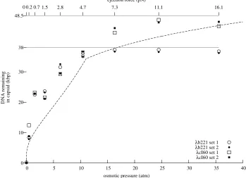
2005a; Grayson et al.2006) to demonstrate that the forces measured during packaging were also present

during ejection: up to 20 atm of external pressure was required to preventλDNA from beginning to exit

the capsid. We will discuss these experiments in detail in Section 3.1. With an understanding of the internal

force in hand, it is natural to try to visualize the dynamics of the entire ejection process. This was done

using an in vitroreal-time fluorescence assay on phage T5 adhered to a microscope coverslip (Mangenot

et al.2005), and the same general technique also was applied toλ(Graysonet al. 2007). We will discuss

that experiment in detail in Section 3.2. The main result of these experiments is that phage DNA can exit a

pressurized capsidin vitroat a high rate of∼60 kbp/s. However, the situationin vivois more complicated.

In fact, since the pressure within the phage capsid drops to zero as the DNA exits, this pressure will never be

enough to push in the entire phage genome against the cytoplasmic osmotic pressure of the host (∼3 atm).

Specific molecular motors such as RNA polymerase have been implicated in genome transport for phage T7

andφ29(Molineux 2001; Kempet al.2004; Gonz´alez-Huiciet al.2004), but it is not clear which motors are used for other phages, such asλ. In Section 3.3 we will discuss an attempt to observe the ejection process

in vivoforλ.

1.2 The phage ejection problem: how does the DNA get out?

The goal of this thesis is to clarify the physics of DNA ejection from bacteriophages, using phage λas

a specific example to study many aspects of the problem. It is arranged as follows: Chapter 2 develops

quantitative models that predict the forces encountered by the DNA during the ejection process: forces due

to internal pressure (Section 2.1), dynamic friction as the DNA exits the capsid (Section 2.2), and drag from

water rushing into the cell through the phage tail (Section 2.3). Chapter 3 explains in detail experiments

that have been performed on λ in order to test these models and inspire new theoretical developments:

static measurements of ejection pressure (Section 3.1), in vitro single-molecule observations of ejection

(Section 3.2), DNA packaging (Section 3.4), andin vivosingle-molecule ejection observations (Section 3.3).

Chapter 4 discusses the implications of this work for λand other viruses, suggesting avenues for further

research. Chapter 5 is a list of people and organizations who have helped directly and indirectly with this

(13)

Chapter 2

Models of bacteriophage

λ

DNA ejection.

This chapter focuses on theoretical models of the DNA ejection process inλ, a specific part of theλlifecycle

that is accessible to a variety of quantitative experiments. The unifying feature of our approach is that we

are interested in the forces that are present during the ejection process and the effect that the forces have on

the phage lifecycle. Even though a bacteriophage is very large compared to, say, an enzyme, its geometric

regularity on the nm scale suggests that it will be possible to apply straightforward mathematical modeling

to calculate the forces and predict their effects on the ejection process.

There are three reasons to believe a driving force is required to transfer DNA from a phage capsid,

across the cell membrane, and into the cell. First, the DNA must somehow penetrate the membrane, which

is not generally permeable to DNA. Whether this involves a specific channel or a simple puncture of the

membrane is not known. Second, the DNA must overcome roughly 3 atm of osmotic pressure within the

cell, or the DNA will be pushed out. Third, friction acts in opposition to the motion of the DNA, so some

force is necessary to transfer the DNA in a reasonable amount of time.

But what is the source of this force? The traditional model of DNA ejection says that is is simply the

pressure from compressed DNA—this is the picture that we will explore in Section 2.1. We will proceed

to estimate the speed with which the DNA can exit a capsid under this force in Section 2.2. However, in

the case ofφ29and T7, detailed experiments have proven that there is something else responsible for the motion: an energy-consuming motor within the cell (Molineux 2001; Kemp et al. 2004; Gonz´alez-Huici

et al. 2004). Whether this kind of motor is used inλ has not yet been established. It should be noted

that the differences in the DNA ends between the different phages may put different requirements on DNA

import. However, it is clear that for most phages some additional force will be required to overcome the

(14)

level. Section 2.3 is a detailed exploration of one model that can account for the translocation of the genome

against a cytoplasmic osmotic pressure.

We will base our models on phage λ, a typical tailed phage with a dsDNA genome, similar to the

majority of phages found in the environment (Fil´eeet al.2005). The genome of phageλis a single 48.5 kbp

piece of DNA with complementary 12 bp overhangs at each end: upon genome transfer into a host cell, the

complementary ends adhere, forming a plasmid-like circle of DNA from which genes can be transcribed.

The genome is stored within an icosahedral capsid with an inner surface we will approximate by a sphere:

model-based interpretation of X-ray scattering data puts the inner radius at 29.4 nm (Earnshaw and Harrison

1977), while a cryo-EM imaging study found approximately 27.5 nm (Dokland and Murialdo 1993). Not

knowing which experiment is likely to be more accurate, we will average the two values and use the radius

Rcapsid ≈28.5±1nm. DNA translocation takes place through a tail of lengthLtail ≈100nm. The radius

of the inside of the tail is unknown, but we will chooseRtail ≈2nm as a reasonable value for the purposes

of making estimates.

Some other physical constants will be important for the calculations in this section. DNA is modeled as

a cylinder of radiusrDNA = 1nm and length 0.34 nm/bp, with persistence lengthξ = κ/kBT = 50nm,

whereκis its flexural rigidity. The viscosity of water will play a role in understanding hydrodynamic drag;

at 37◦C, it has a value ofη = 0.7centipoise = 7×10−4N s m−2 = 7×10−10pN s nm−2. We will take

kBT = 4.28pN nm at 37◦C. Typically, experiments are performed withλin a buffered salt solution: we

will assume that the density of cations in solution is 10 mM.

Though we focus on λ in our calculations, this is just for specificity and for our later application to

experiments: it is important to keep in mind that the techniques we describe may be equally well applied to

any phage, by modifying the numbers given above and recalculating the predictions.

2.1 Theoretical model of internal pressure

One source of driving force is the pressure within theλcapsid caused by highly compressed DNA. There

are at least four pieces of evidence that the DNA pressure is critical to the survival ofλ:

• There is a maximum amount of DNA that can be packaged into aλcapsid (Feisset al. 1977). This

is unsurprising, since the capsid size is fixed, and at some point either the motor will not be strong

(15)

[image:15.612.218.408.78.295.2]

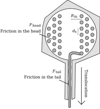
Figure 2.1: Diagram of a bacteriophage λ capsid. Three important dimensions are marked: Rcapsid ≈

28.5 nm represents the inner radius of the head, where the genome is stored; Rtail ≈ 2 nm is the inner

diameter of the tail tube through which the DNA is translocated (this value is unknown); andLtail ≈100nm

is the length of the tail.

Figure 2.2: The inverse-spool model of DNA packaging in a bacteriophageλcapsid, in cross section. The circles indicate the DNA genome, wound many times around the capsid, from the outside to the inside, terminating at an inner radiusRin. The DNA forms a hexagonal lattice with spacingds; the internal energy

[image:15.612.202.401.388.605.2]

(16)

• There is a minimum amount of DNA required in aλcapsid, which is not due to the necessity of any

particular genes for reproduction (Feisset al. 1977). In fact, arbitrary DNA may be used to reach

the minimum. This may be due to an inability of the phage to inject its DNA into the cell when the

internal pressure is too low.

• Phages with long genomes have a strict requirement of Mg2+ ions for survival—this is almost

cer-tainly due to the pressure-reducing effect of Mg2+; without it, the capsids may explode (Parkinson

and Huskey 1971).

• DNA condensing ions such as spermine causeλphages to lose their infectivity. Since DNA

conden-sation involves increasing attractive forces between the DNA, it stands to reason that the effect on a

phage capsid is to reduce the internal DNA pressure, and if the pressure is necessary for infection, this

reduction in pressure could cause a loss of infectivity (Katsura 1983).

2.1.1 Goals for the model

The arguments about pressure within the phage capsid presented in the previous section must be made more

specific for us to proceed. What we mean when we say that internal pressure drives ejection is precisely

that there is a free energyGconf associated with the conformation of the DNA within a phage capsid, and thatGconfis an increasing function of the lengthLDNAof the packaged DNA. As the DNA exits the capsid,

LDNAdecreases, and we derive a force driving the ejection

Fconf= +

∂Gconf(LDNA, Vcapsid)

∂LDNA

, (2.1)

where the positive sign indicates that the force is directed into the host cell. Our objective is to make

quantitative predictions for the relationship

LDNA−→Fconf

for bacteriophageλunder conditions corresponding to the experiments described in Section 3.1. In fact, our

primary goal in developing the model is to compare its predictions to our experimental results, so we will

make sure it is both

(17)

(b) minimal, in that we will leave out effects that are poorly understood or too small to be tested.

To satisfy (b), we will first derive three simple models: two that just take the interaxial electric forces

into account ( Sections 2.1.2 and 2.1.3), and one that only takes DNA bending elasticity into account

(Sec-tion 2.1.4). We will conclude (Sec(Sec-tion 2.1.5) by comparing all three models in light of the precision of

experimentally-accessible data to find our minimal and complete model.

2.1.2 Simple model I: counterion entropy

A first step toward understanding pressure withinλis to compute how much of the internal volume of the

capsidVcapsidis taken up by theλgenome. Specifically, we are interested in the quantity

α= VDNA

Vcapsid

= πr

2

DNALDNA

4

3πRcapsid3

= 5.2×10

4_nm3

9.7×104_nm3 = 0.53. (2.2)

We see that about 50% of the space inside ofλis taken up by DNA. This number is approximately the same

for all tailed phages, as shown in Table 2.1.2, while viruses that infect eukaryotic cells typically have a much

smaller value ofα. The following model shows thatα≈0.5, together with some very basic considerations, directly implies a pressure of tens or hundreds of atmospheres.

Experimentally, phage λmust always be suspended in a buffer solution containing both positive and

negative ions; the positive ions, in particular, are necessary to balance the negative charge (2 e−/bp) of DNA. Since 50% of the space in the capsid is taken up by DNA, the remaining 50% is filled with water

and counterions. Since the phage capsid is porous (except perhaps in the case of T4), counterions will be

exchanged freely with the experimental buffer. The volume of a base pair of DNA isVbp =πrDNA2 ·0.34nm,

so the counterion density is

ρ= 2e−/qionVbp, (2.3)

whereqionis the charge of the positive counterion. For Na+, we haveρ = 2nm−3, or 3.3 M. The entropy

ofN ions in a volumeV is approximated by

S=kBlogVN, (2.4)

so that the pressure is

T∂S(N, V) ∂V =

N

(18)

Host Virus Type Diameter (nm) Genome (kbp) α(%) Spacing (nm)

Bacteria λwt dsDNA 57 48.5 53.4 2.61

T7 dsDNA 55 40 49.0 2.72

φ29 dsDNA 44.1 19.3 45.9 2.81

λb221cI26 dsDNA 57 38 41.9 2.94

MS2 ssRNA 23 3.6 23.3 2.76

Eukarya poliovirus ssRNA 27 7.4 29.8 2.44

CCMV ssRNA 20.8 3.2 28.2 2.51

west nile ssRNA 34 11 22.2 2.83

HIV ssRNA 70 18.4 4.3 6.43

smallpox virus dsDNA 220 186 3.6 10.04

mimivirus dsDNA 400 800 2.6 11.81

SARS ssRNA 100 29.8 2.4 8.61

Table 2.1: Packing of the genome into various bacterial and eukaryotic viruses. For each virus, the table shows the capsid radius (averaged to give the correct volume for non-spherical viruses), genome type and size, the inferred fraction of space taken up in the capsid, α, and the resulting spacing between strands, assuming hexagonal packing throughout the interior. What we see here is that the tailed phage all have

α ≈ 50%, while RNA phages and eukaryotic viruses tend to have much lower values ofα. References for λ: Feiss et al. (1977); Earnshaw and Harrison (1977); Dokland and Murialdo (1993); T7: Cerritelli

et al.(1997); φ29: Taoet al.(1998); MS2: Koninget al.(2003); poliovirus: Lentzet al.(1997); CCMV:

(19)

which is the familiar expression for the osmotic pressureΠ. We have

ΠNa=ρ·kBT = 2nm−3·4pN nm= 8.0pN nm−2= 79atm. (2.6)

Alternatively, for Mg2+, we find an osmotic pressure reduced by a factor of two, to 40 atm.

The intent of the preceding estimates is to give us a feeling for the high concentrations and pressures

found within a phage capsid. Strictly, what the partial derivative in Equation 2.5 means is that this pressure

quantifies howGconfchanges if the capsid volume is changed without a concurrent change in the number of counterions. One way that the volume accessible to counterions can increase is if the DNA is translocated

into the capsid, say by a distance∆x. The change in accessible volume is given byπ r_DNA2 ·∆x. This means that we multiply8.0pN nm−2by the cross-sectional area of DNA to findFconf= 25pN, an estimate for the scale of the force that the pressure applies to the DNA at the beginning of genome translocation. However,

as the DNA exits the capsid, the number of counterions within the capsid will change. We must add terms to

Fconfthat take into account the change inGconf with respect to the number of counterions. In the language of thermodynamics, these terms represent the difference in chemical potential encountered by the ions as

they exit the capsid.

To estimate the force more precisely, we consider a system of N ions, with N1 found in a volume

of water V1 within the capsid, and N2 found in a volume of water V2 outside of the capsid. Following

Equation 2.4, the numbers of arrangements of the ions inside and outside of the capsid areVN1

1 andV

N2

2 ,

respectively. An additional factor _NN

1

accounts for the number of possible choices for which ions are found

within the capsid, giving us an expression for the total entropy:

S =kBlog

N N1

VN1

1 V

N2

2

≈kBlog

NN1

N1N1

VN1

1 V

N2

2

. (2.7)

We compute the force on the DNA by differentiating the free energy with respect to the lengthLDNAof the

DNA left inside the capsid:

Fconf=−T

dS dLDNA

≈ −kBT

dN1

dLDNA

logN − dN1

dLDNA

logN1 (2.8)

+ dN1

dLDNA

logV1−

N1

V1

·πr2_DNA− dN1

dLDNA

logV2+

N2

V2

·πr2_DNA

(20)

which we can rewrite conveniently as

Fconf =T

dS dLDNA

≈kBT

dN1

dLDNA

logρ1

ρ + (ρ1−ρ)·πr

2 DNA

, (2.9)

whereρ is the concentration of counterions outside of the capsid andρ1 is the concentration inside. The

force is positive,i.e., directed out of the capsid, and made up of two terms. The first corresponds to the force

required to transport ions against a chemical potential difference, while the second is the pressure-area force

that we calculated earlier. In terms of the parameters relevant toλ, we have

dN1

dLDNA

= 2e −

qion·0.34nm

; (2.10)

ρ1 =

2e−LDNA/qion/0.34nm

Vcapsid−πrDNA2 LDNA

. (2.11)

It is apparent that as DNA leaves the capsid, the pressure will decrease. A plot of the quantitative predictions

of this model is shown in Figure 2.4. What we see from this plot is that forces of 100–200 pN are predicted;

the shape of the curve is dominated by the logarithmic chemical potential term. In fact, by completely

ignoring the three-dimensional arrangement of the ions inside and outside the capsid, we are missing some

important details that reduceFconf to a fraction of this value. Theoretical treatments such as the Poisson-Boltzmann approximation or the theory of condensation by Manning (1969) would take into account the fact

that some ions remain close to DNA after its exit from the capsid, reducing the entropy gain from exiting

DNA. However, for a variety of reasons, first principles models of the pressure within tightly-packaged DNA

do not give very accurate results when compared to real-world data. Perhaps the most important is the fact

that the discrete nature of the ions is ignored in continuum statistical mechanics approximations. Ion-ion

interactions and the particular locations of the charged phosphate groups on the DNA backbone are both

difficult to model in a simple theory. A Monte Carlo simulation technique by Lyubartsev and Nordenski¨old

(1995) was successful in taking these features into account, but the effects of large-scale bending fluctuations

in the structure of DNA itself could not be included.

2.1.3 Simple model II: empirical interstrand forces

Beyond theoretical calculations, the most reliable numbers come from measurements on bulk DNA,

com-pressed by osmotic pressure (Rauet al.1984; Parsegianet al.1986; Podgorniket al.1995; Streyet al.1997,

(21)

into hexagonally packed liquid crystals, as a function of the interstrand spacingds(See Figure 2.2.) A main

result of this body of work is that the dependence fits well to an exponential in the relevant range for phage

packaging:

Π = Π0e−ds/c, (2.12)

where Π0 is the hypothetical pressure at zero spacing, andc is a decay constant that corresponds to the

length scale of the interactions between the DNA strands. The free energyGof DNA in the capsid is given

by integrating the forces required to assemble it from infinity:

G= Z ∞

ds

Π∂Vcapsid(LDNA, ds)

∂ds

d(ds) = √

3·Π0e−ds/c·LDNA

cds+c2

. (2.13)

In working with these expressions, note that for hexagonal packing of a lengthLDNAinto a volumeVcapsid,

√ 3 2 d 2 s = Vcapsid LDNA ; (2.14)

∂ds(LDNA, Vcapsid)

∂LDNA

=− ds

2LDNA

. (2.15)

Using these expressions can derive a force for inserting DNA from bulk solution into a phage capsid: it is

given by the derivative of the free energy

∂G(LDNA, Vcapsid)

∂LDNA

=

√

3 2 ·Π0e

−ds/c

d2_s + 2cds+ 2c2

. (2.16)

There are three terms in Equation 2.16: thed2_s term is what you get if you na¨ıvely multiply the pressure by

the effective areaVcapsid/LDNA of the DNA in the capsid, while the other two terms have to do with the

interaction energy of additional DNA with its neighboring strands (about 25% of the total of all three terms.)

Equation 2.16 was used to calculate the forces from the parametersΠ0andcin previous work (Purohitet al.

2003, 2005; Graysonet al.2006).

The values of the parametersΠ0 andccan be extracted from the measurements of Rauet al.. But how

accurately can we know these parameters? One way to address this issue is to use the variations found

in pressure measurements taken under slightly different buffer conditions, at different times, by different

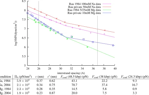
experimenters. Figure 2.3 shows several sets of X-ray scattering data under different conditions.

(22)

dependence and another with a higher value ofc. Since the force is derived from an integral over all DNA

spacings, this will have an effect, especially at low packing fractions. Let us define the two exponential

regimes as: Π =     

Π0e−ds/c ifds< a;

Π0₀e−ds/c0 _otherwise.

(2.17)

Here we set

Π0₀ = Π0e−a/c+a/c

0

(2.18)

to ensure that the function is continuous. With this new formula, we can recalculate:

Gconf=              √

3·Π0e−ds/c·LDNA

cds+c2

−√3·Π0e−a/c·LDNA

ca+c2

+√3·Π0₀e−a/c0 ·LDNA

h

c0a+c02i ifds< a; √

3·Π0₀e−ds/c0 _·_L

DNA

h

c0ds+c02

i

otherwise.

(2.19)

Fconf =              √ 3 2 ·Π0e

−ds/c_d2

s + 2cds+ 2c2

−√3·Π0e−a/c·

ca+c2

+√3·Π0₀e−a/c0·hc0a+c02i ifds< a;

√

3

2 ·Π

0

0e−ds/c

0h

d2_s + 2c0ds+ 2c02

i

otherwise.

(2.20)

Note that the equations imply thatFconfis a continuous function ofds, despite the change in parameters at

ds = a. The value ofds can be found as a function ofLDNAandVcapsid from Equation 2.14. Figure 2.3

shows our fits to the various sources of experimental data on DNA packing, together with predictions from

the present model forλ. What we see is a 30–60% variation ofFconf, depending on the source of the data used in fitting. This is due to differences in buffer conditions and also probably systematic errors in the

experimental techniques, which differ slightly between the datasets. We have chosen the parameters derived

from the more recent datasets for use in further calculations, including the plot ofFconfshown in Figure 2.4.

2.1.4 Simple model III: only bending energy

So far we have considered the energy required to bring strands of DNA in a closely packed arrangement.

(23)

5 5.5 6 6.5 7 7.5 8 8.5

24 26 28 30 32 34 36 38 40

log10(P/(dyne/cm

2 ))

interstrand spacing (A)

Rau 1984 100mM Na data Rau private 50mM Na data Rau 1984 5/25mM Mg data Rau private 10mM Mg data

Condition Π0(pN/nm2) c(nm) c0(nm) Fconf(48.5 kbp) (pN) Fconf (38 kbp) (pN) Fconf(24.3 kbp) (pN)

Na, 1984 5.9×103 0.37 0.62 43.1 22.2 9.3

Na, 2004 2.1×104 0.34 0.75 70.7 37.4 16.7

Mg, 1984 2.3×104 0.28 0.35 14.5 5.8 0.9

[image:23.612.85.584.189.506.2]

Mg, 2004 1.9×105 0.23 0.87 20.0 7.5 3.3

Figure 2.3: Pressure vs. spacing data from Rau and Parsegian. Some of the sets were privately communi-cated to me (2004) for salts in the presence of 10mM TRIS, some were taken from the plots in Rauet al.

(1984). Parameters were extracted using exponential fits to the data from 24–32 nm. The vertical gray lines correspond to thedsvalues forλwhen 100% and 50% of the DNA is packed. For these spacings the forces

(24)

bent to fit into the capsid (Garciaet al.2007), so there is an additional energy that should be considered: the

bending energy of DNA, which is given in (Boal 2002):

∆Ebend = ∆L· 1

2ξkBT R

−2_, _(2.21)

whereR is the radius of curvature of a lengthL of DNA. Let us consider a model in which the capsid is

filled uniformly with a lengthLDNAof DNA, but only the bending energy contributes toFconf. Following Purohitet al.(2003), we will assume that the DNA is packed into an inverse-spool, though a ball-of-twine

model in which the axis of spooling varies with radius could lead to a slightly smallerFconf(calculation not shown). For an inverse spool, the total bending energy is given by an integral of Equation 2.21 over the

volume of the capsid, which can be thought of as a sum of many concentric cylindrical shells of DNA of

area4πrqR2_capsid−r2_{. We will assume the DNA is packed down to an inner radius of}_R

in, which gives

the following expression for the total energy:

Ebend =

ξkBT

2

Z Rcapsid

0

4πrqR2

capsid−r2r

−2 L

Vcapsid

dr (2.22)

= 4πξkBT LRcapsid

2Vcapsid ·

log R

Rin

+ logq1−R2

in/R2capsid

−q1−R2

in/Rcapsid2

(2.23)

≈ ξkBT L

2 ·(0.33·Rcapsid)

−2_, _(2.24)

where we have obtained the final approximation by putting in a value of 1 nm forRin, representing the

absolute limit of DNA bending. (The result is very weakly dependent onRin.) What this expression means

is that DNA has the same bending energy that it would have if it were all bent at an “average” radius of

0.33·Rcapsid. This means that DNA feels a force during translocation of

Fconf =

dEbend

dL = ξkBT

2 ·(0.33·Rcapsid)

−2_≈₁_.₂_pN_. _(2.25)

This value is an upper bound for the contribution of DNA bending stiffness toFconf: according to the inverse spool model, at low packing fractions the DNA arranges itself around the outer surface of the capsid, with

a higher average radius than for a fully packed capsid, so we would expect the bending force to be lower.

However, as shown in Figure 2.4, the value of 1.2 pN is so low that we don’t expect it to play any important

(25)

2.1.5 Comparison of the models

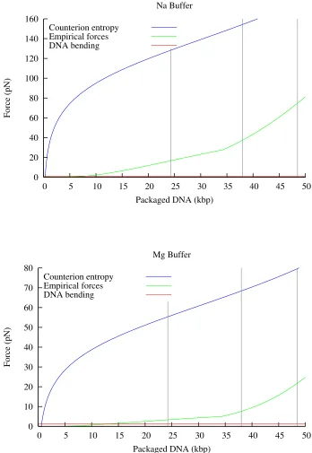
Figure 2.4 compares the models derived in the previous three sections. What we can see from this graph is

that the model based on counterion entropy alone (Model 1) gives much higher predictions forFconf than the model based on empirical measurements of DNA (Model 2). Most of the difference between these two

models appears during the first 10 kbp of DNA packaging, due to the rising chemical potential difference as

the concentration of ions within in the capsid approaches molar levels. Model 3, taking into account only

the bending energy, predicts a relatively much smallerFconf, which only exceeds Model 2 when less than about 10 kbp is packaged. At these low packing fractions, the bending force is actually an overestimate,

since the DNA is able to rearrange, causingRinto be much larger. More detailed models allowRinto vary,

effectively combining Models 2 and 3 to compute a energy-minimizing arrangement for the capsid (Purohit

et al. 2003, 2005). However since the contribution of the bending energy to the force is so small, these

models do not predict a significantly different force from Model 2 alone. Model 2 will be used to calculate

(26)

0 20 40 60 80 100 120 140 160

0 5 10 15 20 25 30 35 40 45 50

Force (pN)

Packaged DNA (kbp) Na Buffer

Counterion entropy Empirical forces DNA bending

0 10 20 30 40 50 60 70 80

0 5 10 15 20 25 30 35 40 45 50

Force (pN)

Packaged DNA (kbp) Mg Buffer

[image:26.612.127.475.81.586.2]

Counterion entropy Empirical forces DNA bending

(27)

2.2 Modeling the mobility of DNA during ejection

Section 2.1 explained how pressure produced by the confined DNA within a phage capsid leads to a force

Fconfduring translocation. Other forces may affect translocation: for example a forceFosmoriginates from internal osmotic pressure in the host cell. To a student of freshman physics, it is tempting to add up all of

the forces and apply Newton’s law. Suppose the total force isF = 1pN. Using the mass of theλgenome, we find the acceleration

dv dt =

F m =

1·10−12N

5·10−20_kg = 2·10

7_m_/_s2_. _(2.26)

Clearly such an acceleration can’t continue for very long: like all macromolecular systems, the DNA will

be constrained by molecular-scale friction. Instead of acceleration, we have a force balance:

Fconf+Fosm+Ffric(v) = 0. (2.27)

It is not clear how to address friction at the molecular level. However, since the DNA is in a fluid state (Strey

et al.1997), we expect the frictional forceFfric(v)to behave like macroscopic hydrodynamic drag,

increas-ing with velocity. In fact, it will be useful to assume a linear dependence:

Fconf+Fosm−v/µ= 0, (2.28)

whereµ, which we call themobility, characterizes the frictional force. The problem of modeling friction

during DNA ejection is thatµdepend on the configuration of the DNA. With one exception (Z´arybnick´y

1969), theoretical papers have avoided explicitly estimating the friction, focusing instead how the friction

should scale with parameters like the concentration of DNA within the capsid (Gabashvili and Grosberg

1991, 1992; Spakowitz and Wang 2005; Inamdaret al.2006). However, Section 3.2 describes an experiment

that can make a direct measurement ofµ, demanding a theoretical interpretation. This section aims to satisfy

that demand with several quantitative estimates ofµ.

2.2.1 Friction in the phage tail

In this section we discuss the drag that is experienced by the DNA as it translocates through the tail, due to

friction in a hypothetical layer of water between the DNA and the inner wall of the tail. The method of this

(28)

We begin by assuming that the pore opened by the phage is a annular tube: it is bounded by the DNA

on the inside and the tail proteins on the outside. The general solution for cylindrically symmetric flow with

an inner boundary atrDNAis a standard result; see, for example, Weisstein (2005). The flow velocityuis a

function only ofr, given by:

u(r) =u(rDNA)−

Q

4ηLtail

r2−r_DNA2 −clog(r/rDNA)

. (2.29)

HereQrepresents the pressure difference along the length of the tail. In the case of DNA translocation at

velocity v, the boundary conditions are thatu(rDNA) = v andu(Rtail) = 0, resulting in a value for the

constantcof:

c= R

2

tail−rDNA2 −v· 4ηLtail

Q logRtail/rDNA

. (2.30)

The shear force exerted by the water on the DNA is given by

Ftail = 2πrDNALtailη

du

dr =−πrDNA Q

2 (2rDNA−c/rDNA) . (2.31)

Substituting the value ofcfrom Equation 2.30 and expanding the result, we find

Ftail =−πrDNA

Q

2

2rDNA−

R2

tail−rDNA2

rDNAlogRtail/rDNA

− v·2πηLtail

logRtail/rDNA

. (2.32)

Notice that Equation 2.32 consists of two terms: one that is linear in the pressure differenceQand one that

is linear inv. Using the values given earlier forη,Rtail,rDNA, andLtail, we find

Ftail = 3.7nm2·Q−2.2×10−4 pN·s

kbp ·v . (2.33)

We will examine the meaning ofQin Section 2.3; for now, let us assume thatQ= 0. Under the assumption that the tail provides the only source of friction, we find

µ= 4500 kbp

s·pN. (2.34)

What should be recognized in this case is thatµis independent of the configuration of the DNA: it will be a

constant throughout the translocation process. Also, it should be understood that under this approximation,

(29)

other predictions for the mobility in Figure 2.5.

2.2.2 Friction in the phage head

Gabashvili and Grosberg (1991) suggested three sources of friction for genome translocation: friction in

the tail, friction between the DNA and the inner surface of the phage head, and friction between

neighbor-ing sections of DNA in the head. Section 2.2.1 focused on the first source of friction; in this section we

will make an estimate of the last, which is caused by DNA sliding past itself as it exits the capsid. In a

hexagonally-packed arrangement, one section of the DNA has six neighbors, separated from it by a water

layer of thicknessds−2·rDNA. As the DNA slides out of the capsid, each of the neighbor sections will

be moving, possibly in different directions. The central section will be subjected to a friction that depends

on how fast the neighbors move: if they move in opposition, the force will slow down translocation, while

if they move together, the force will speed up translocation. We have no way of knowing what the exact

arrangement of the DNA will be as it slides out, so we suggest a reasonable approximation: assume that the

opposing and aligned motions of the neighbor strands cancel out to an average of zero velocity. Then we

can imagine that the central strand is actually moving within a stationary tube of radiusds−rDNA, so the

force can be found with Equation 2.32:

Fhead = −

v·2πηLDNA

log (ds−rDNA)/rDNA

; (2.35)

µ = 1

2πηLDNA

·log ds−rDNA

rDNA

. (2.36)

Here,LDNAis the amount of DNA remaining in the capsid. According to Table 2.1.2, for a fully packedλ

(LDNA= 16µm) we haveds = 2.61nm. These numbers lead to the numerical result

µ= 6.8µm·s−1pN−1 = 20.kbp·s−1pN−1. (2.37)

The friction is about 200 times stronger under this approximation, which makes sense, since the genome

is about 200 times longer than the tail alone. However, as the DNA exits the capsid,LDNAwill decrease,

causingµto increase. The predictions of a mobility model, taking into account only the friction in head, are

(30)

2.2.3 Friction from layer sticking (Grosberg/Rubinstein model)

This section discusses an idea proposed by Rubinstein and Grosberg (2007) to explain experimental

mea-surements of mobility by Graysonet al.(2007) (we discuss the experiments in Section 3.2.) The basic result

of those experiments is thatµis an exponential function of the amount of DNA within the capsid with a

decay constant of L0 ≈ 10 kbp. The suggestion, based purely on the empirical observation of an

expo-nential dependence, is that this could be modeled by hypotheticalstickerson the DNA, spaced at a linear

densityσ on the DNA, that fluctuate between bound and unbound states. When bound, the DNA is “stuck”

and unable to translocate, but when the sticker is unbound, it may translocate freely. Suppose that when it

is moving freely in the head, it has mobilityµ0 = 4500kbp/s·pN given entirely by resistance in the tail.

To understand the implications of this model, we must compute how much time the DNA spends in its free

state.

We model the stickers with the assumption that each has a probability of being unbound given by the

Boltzmann factor:

P1 =

exp(−ε/kBT)

1 + exp(−ε/kBT)

, (2.38)

where ε is the sticking energy. Then the probability for theN = σL stickers to all be simultaneously unbound, allowing the DNA to move, is

P =

exp(−ε/kBT)

1 + exp(−ε/kBT)

σL

. (2.39)

Then the average mobility is given by

µ=µ0·

exp(−ε/kBT)

1 + exp(−ε/kBT)

σL

. (2.40)

Sinceεandσare unknown and probably unmeasurable constants, it will be most useful to rewrite this in a

simpler form:

µ = µ0·exp(−L/L0), with (2.41)

L0 = −σ−1log

exp(−ε/kBT)

1 + exp(−ε/kBT)

. (2.42)

(31)

equalσ−1 under any circumstances. In fact, for the likely situation thatε > kBT, we have

L0 =σ−1ε/kBT . (2.43)

Suppose, for example, sticking corresponds to a typical hydrogen bonding interaction withε/kBT ≈10.

Then we have

σ−1=L0/10≈1kbp. (2.44)

It is not clear what process could cause sticking every 1 kbp. The outer loops of DNA that make contact

with the capsid have sizes of approximately 300 bp, while an entire layer of DNA loops in the inverse spool

model contains about 5–10 kbp.

Alternatively, suppose that every base pair is equally likely to cause sticking:

σ−1 = 1bp; (2.45)

ε/kBT = 10−4. (2.46)

In this case, for the sticking model to be correct, we would have to think of a mechanism by which bases

can cause sticking with a probability of approximately10−4. The usefulness of this model is limited by our inability to think of a physical mechanism for the sticking process. In fact, since the model was just created

as an explanation for the data, we have no particular reason to believe that it accurately represents the reality

of the motion of the phage DNA. For example, it may be that a single loop or layer of DNA may move

without it being necessary for the entire length of the genome to be sliding; these possibilities may or may

not lead to different functional forms forµ. Despite the limitations of this model, its predictions are plotted

(32)

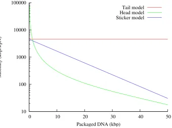
10 100 1000 10000 100000

0 10 20 30 40 50

Mobility (kbp/s/pN)

Packaged DNA (kbp)

[image:32.612.136.476.206.459.2]

Tail model Head model Sticker model

Figure 2.5: Plots of the mobilityµ =v/F of DNA during the translocation process, under three different models, as a function of the amount of DNA within theλcapsid. The red curve takes into account only friction from the tail, giving a constant value forµ(see Section 2.2.1.) The green curve takes into account only friction from within the capsid, which gives a value that changes according to the spacing between the strands (see Section 2.2.2.) The blue curve takes into account only friction from “sticking” points spaced along the DNA, leading to an exponential dependence ofµon L; we have chosen the parameters so that

(33)

2.3 Calculating drag forces in the toilet-flush model

In the preceding sections we have discussed a theoretical model of the pressure within the capsid as well as

the friction that may be encountered during DNA translocation. It is also essential to consider the kinds of

forces that may be encountered whenλis actually ejecting its DNA into a host cell, since the phage/host

interaction may play an important role. Some discussion about the various kinds of effects that may come

into play during DNA translocationin vivois given in Section 3.3. Here we will describe the details of one

source of force that may speed up DNA translocation. The model described in this section is also described

elsewhere (Grayson and Molineux 2007).

2.3.1 Precise definition of osmotic pressure

Because bacterial cells lack a cytoskeleton, they rely on an internal pressure to push the cell membrane

outward. This pressure serves both to help maintain the cell shape and to allow the cytoplasm to increase in

volume as the cell grows. The internal pressure is created by the presence of concentrated solutes within the

cytoplasm, though it is unclear which solutes play the dominant role. Solutes by definition have an affinity

for water, so that there is an free-energy decrease associated with transferring a small volume ∆Vwater of water into the cell,

∆Fosm=−Π·∆Vwater, (2.47)

whereΠis the cytoplasmicosmotic pressure, a number that depends on the concentrations of various solutes in the cytoplasm relative to the extracellular space. This osmotic pressure can be measured in various ways:

Stocket al.(1977) measured the cellular contents ofE. coliunder various osmotic conditions and computed

a theoretical pressure of 0.33 pN/nm2forE. coligrowing rapidly but approaching saturation; Knaysi (1951)

appliedplasmolysis, a contraction of the cytoplasm away from the outer membrane, at various times during

growth of an E. coliculture, finding an osmotic pressure up to 1.5 pN/nm2 during initial rapid growth,

which stabilized at 0.2 pN/nm2. More references and discussion about the osmotic pressure withinE. coli

can be found in Neidhardt (1996), p. 1211. We will takeΠ = 0.3pN/nm2, or 3 atm as a standard value. In the absence of any constraints, water will flow into the cytoplasm, diluting the internal solutes, until the

(34)

pressure, defined by a free energy cost

∆Fhyd=P ·∆Vwater. (2.48)

In this case, water will continue to flow into the cell until an equilibrium is reached where the net free energy

benefit of transferring water is zero; where

P = Π. (2.49)

In many situations, this equilibrium is reached quickly, so there is no need to make a distinction between

osmotic pressure and the resulting hydrostatic pressure.

However, during rapid cell growth, the cytoplasm is clearly out of equilibrium to some extent, since

water is continuously flowing into the cell. In addition, there are various experimental techniques that

involve subjecting a cell to osmotic shocks, causing the cytoplasm to shrink or swell; in these experiments,

the cell is therefore temporarily out of equilibrium. The remainder of this section is concerned with the

problem of quantifying the extent to which the cell is out of equilibrium under these different conditions.

In particular, we will try to quantify the pressure imbalanceQ ≡Π−P, which will be positive whenever water is flowing into the cell, and negative when water is flowing out.

For the following estimates we will assume thatE. colihas a cell volume of0.4µm3 = 4×108nm3. During rapid growth,E. colidivides once every 1200 s. This means that water must flow into the cell at a

rate of

Φ = 4×108nm3/1200s= 3.3×105nm3/s. (2.50)

The pressure imbalance depends on the permeability of the cytoplasmic membrane to water: a more

permeable membrane will allow the cell to stay closer to equilibrium. To estimate this permeability, we

turn to experiments in which measured osmotic shocks cause measurable changes in cytoplasmic volume.

Delamarche et al. (1999) report a water channel, AqpZ, that is present in the cytoplasmic membrane of

E. coli. In their experiments, cells are subjected to hyperosmotic shocks (Q <0), causing a shrinkage of the

cytoplasm, observable under cryo-electron microscopy, known as plasmolysis. From their graphs we see that

a 1 osM (2.6 pN/nm2) shock causes AqpZ+ cells to begin shrinking at a rate of∼0.2cell volumes/15 s= 5.3×106nm3/s, while AqpZ- cells shrink much more slowly, at about6.7×105nm3/s. From this we can infer that AqpZ is the primary water device for water transport across the cytoplasmic membrane, and we

(35)

the influxΦof water andQ:

Φ = Q

2.6pN/nm2 ·5.3×10

6_nm3_/_s₌_Q_·₂_.₁_×₁₀6_nm3_/_s_·_nm2_/_pN_. _(2.51)

The coefficient multiplyingQon the right side of Equation 2.51 is the permeability of the cell membrane

to water; the assumption of linearity allows us to make estimates for other conditions. For example, during

rapid growth, the rate of water influx implies a pressure imbalance of

Q= 3.3×105nm3/s· 2.1×106nm3/s·nm2/pN−1 = 0.16pN/nm2. (2.52)

Is the cell permeability given in Equation 2.51 reasonable? A simple hydrodynamics calculation shows

that it is. Laminar fluid flow through a cylindrical pipe is traditionally calculated using a formula owed to

Poiseuille:

Φ = Q

l π

8ηr

4 ₌_Q_·₁_.₄_×₁₀4_nm3_/_s_, _(2.53)

usingl = 2nm andr = 0.15nm as the length and radius of the AqpZ pore. This would imply that about 150 copies of AqpZ are required to give the cytoplasmic membrane the permeability given in Equation 2.51,

which is a very reasonable number for a membrane channel.

2.3.2 Implications of the toilet-flush model

The key result of the previous section is that the osmotic pressure imbalanceQofE. colicauses an influx

of water through all open channels. As we assumed already in Section 2.2.1, whenλbinds toE. coliit also

opens a channel through which water can flow: the space between the DNA and the inner surface of the tail.

This inrush of water will apply a force to the DNA, speeding up translocation into the cell.

Our goal is to compute the ratevat which DNA is translocated into the cytoplasm, in units of kbp/s, as

a function of the amount of DNA that has been translocated. The value ofvcan be compared to experiments

that quantitatively measure the translocation process. The basic equation that we will use to determine the

dynamics of the system is a balance of forces:

Fconf+Fosm+Ftail(v) = 0, (2.54)

(36)

respectively. The functionFtail(v) is the force due to water flowing between the tail and DNA. We have shown in Section 2.2.1 thatFtail reduces to a linear function of the pressure differenceQandv:

Fconf+Fosm+ 3.7nm2·Q−2.2×10−4 pN·s

kbp ·v = 0. (2.55)

Using the value ofQfrom Equation 2.52, we get a value of0.59pN for the pressure-dependent term of

Ftail. For the valueΠ = 0.3pN/nm2that was quoted earlier, we find thatP = 0.14pN/nm2, much reduced from its equilibrium value. This allows us to estimateFosm =P ·πr2DNA =−0.44pN. The force balance

of Equation 2.33 now becomes

v= Fconf+ 0.15pN

2.2×10−4_pN_·_s_/_kbp =Fconf·4500

kbp

pN·s+ 680kbp/s . (2.56)

This model predicts extremely high velocities for DNA translocation intoE. coli, suggesting that the DNA

may be completely translocated into the cell in less that 0.1 s. However, we have made numerous

assump-tions in our calculaassump-tions, so that our numbers can easily be off by an order of magnitude. For example, the

thickness of the gap between the DNA and tail is not accurately known, and it varies along the length of the

tail. A gap of 0.3 nm, for example, enough for just one layer of water, would result in a prediction that the

term ofFtaildepending onQis not high enough to overcomeFosm; in this case additional source of energy would be required for translocation of the entire genome. We have also completely ignored the fact that

water itself is discrete on the nanometer scale, so that describing its flow with a continuum fluid dynamics

model is somewhat absurd. However, in the absence of better experimental data on the flow through

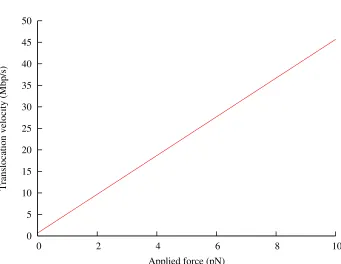
phage-induced channels, the continuum approximation is the best that we have. Figure 2.6 shows the translocation

velocities predicted by this model for forces in the range of 0–10 pN.

The translocation speed at Fconf = 0, 680 kbp/s is fast enough to be consistent with all experiments on phage ejection in vivo: no phage has ever been observed to eject its DNA faster than that. There are

cases, such as T7, in which the DNA is observed to enter the cell much moreslowly; this can be attributed

to mechanisms that slow down the motion of the DNA, such as a constriction region in the channel causing

direct channel-DNA interaction (Kempet al.2004).

The only source we used for the permeability of cell membranes is the study by Delamarcheet al.(1999).

A further study, using real-time fluorescence and light scattering measurements, concluded that plasmolysis

(37)

0 5 10 15 20 25 30 35 40 45 50

0 2 4 6 8 10

Translocation velocity (Mbp/s)

[image:37.612.132.473.211.475.2]

Applied force (pN)

(38)

2005). It is unclear why there is such a huge discrepancy between the two results, but such a highly

perme-able cell membrane would make the forces computed in this paper entirely negligible. The former paper is

more satisfying, both because of its single-cell images that reveal exactly what is happening in the

experi-ment, and because it provides a natural explanation for why bacterial cells must be highly pressurized. It is

also worth mentioning that, according to our calculations, the AqpZ- mutants of Delamarcheet al.(1999)

should not be able to grow as rapidly as the wild-type, unless they have an internal osmotic pressure of at

least1.6pN/nm2= 16atm.

We assumed 0.3 pN/nm2 for the osmotic pressure inside of a cell without much comment, but, as was

discussed, it may be five times higher during rapid growth, presenting a much higher force resisting DNA

entry.

To conclude, we have thoroughly considered the motion of water molecules entering the cytoplasm

through a phage-induced channel. It appears that forces from hydrodynamic drag may be a significant

contributor to the total force on the DNA, and that they are potentially responsible for translocation of the

entire genome. In estimating these forces, it is essential to understand the difference between hydrostatic and

osmotic pressures, which will not be equal in non-equilibrium situations. In any case, there are numerous

unknown quantities in the estimates, and it is hard to draw strong conclusions about the role of hydrodynamic

drag. Experiments to examine these hydrodynamic forces, and non-equilibrium osmotic pressure in general,

(39)

Chapter 3

Experiments on the bacteriophage ejection

process

It is the author’s strong belief that for biology, theory and experiment must go together. A good theory

makes predictions for quantities that can be tested experimentally, which is why Chapter 2 makes a series

of specific predictions, without any free parameters. Even when the parameters are unknown, it is important

to make reasonable estimates, so that it is possible to identify theories that make completely unreasonable

predictions. Similarly, it is essential for experimenters to design experiments to give quantitative results that

can be directly compared to theory. In this chapter we describe a series of experiments onλthat complement

the theoretical models. With the model set by Luria and Delbr¨uck in mind, we hope that for some of the cases

agreement between theory and experiment will clarify our understanding of how phages work. Specifically,

we have carried out an experiment (Section 3.1) to test the pressure estimates of Section 2.1; an experiment

(Section 3.2) that measures the velocity of DNA ejection fromλin vitro, for comparison to the estimates

of mobility in Section 2.2; and we have made progress on an experiment to visualize the ejection process

in vivo (Section 3.3) for comparison to models such as the one presented in Section 2.3. In Section 3.4,

we discuss a comparison of our results on the ejection process with measurements on DNA packaging in

phages.

3.1 Experimental measurement of ejection force

(40)

[image:40.612.139.476.74.434.2]

Figure 3.1: Experimental measurement of ejection force. A. LamB binds to phage tails, triggering the ejection of DNA. The ejection reaches an equilibrium when the internal force balances the osmotic force due to PEG. B. DNase I cuts the ejected DNA into small fragments. C. Phages are removed by centrifugation, leaving the ejected fraction of the DNA in solution. See Section C.7 for the details of the procedure.

bring the accuracy to the level where the quantitative theory of Section 2.1 may be tested. Most generally,

the model predicts thatFconf is a function only of the amount of DNA within the capsid; what this means is that the original genome size of the phage should not affectFconf. A fortuitous feature ofλis that there are mutants available with different genome sizes: in this experiment, we usedλcI60, which has a wild-type

genome length of 48.5 kbp, andλb221cI26, with a genome length of approximately 38 kbp (Feisset al.

1977). See Section C.3 for the technique we used to accurately measure the length ofλgenomes.

The experimental procedure is described in detail in Section C.7 and is illustrated in Figure 3.1.