Image Compression Using a New Technique by
Artificial Neural Network
MOHD. MUNNAZAR ANSARI
Department of E.I.C.
AIET Lucknow (U.P.) INDIA
ATUL MISHRA
Department of Computer Science & Engineering
BBD University Lucknow (U.P.) INDIA
Abstract—In this paper a neural network based image compression method is presented. Neural networks offer the potential for providing a novel solution to the problem of data compression by its ability to generate an internal data representation. This network, which is an application of back propagation network, accepts a large amount of image data, compresses it for storage or transmission, and subsequently restores it when desired. A new approach for reducing training time by reconstructing representative vectors has also been proposed. Performance of the network has been evaluated using some standard real world images.
Keywords—Artificial Neural Network, Image Processing (ANN), Multilayer Perception (MLP), Back Propagation network
INTRODUCTION
Neural networks are inherent adaptive systems. They are suitable for handling non stationeries in image data. Artificial neural network can be employed with success to image compression. The advantages of realizing a neural network in digital hardware are:[2]
Fast multiplication, leading to fast update of the neural network. Flexibility, because different network architectures are possible.
Scalability, as the proposed hardware architecture can be used for arbitrary large network, considered by the no. of neurons in one layer. The greatest potential of neural networks is the high speed processing that is provided through massively parallel VLSI implementations. The choice to build a neural network in digital hardware comes from several advantages that are typical for digital systems:[2] Low sensitivity to electric noise and temperature. Weight storage is no problem.
The availability of user-configurable, digital field programmable gate arrays, which can be used for experiments. Well-understood design principles that have led to new,
powerful tools for digital design The crucial problems of neural network hardware are fast multiplication, building a large number of connections between neurons, and fast memory access of weight storage or nonlinear function look up tables.
The most important part of a neuron is the multiplier, which performs high speed pipelined multiplication of synaptic signals with weights. As the neuron has only one multiplier the degree of parallelism is node parallelism. Each neuron has a local weight ROM (as it performs the feed-forward phase of the back propagation algorithm) that stores, as many values as there are connections to the previous layer. An accumulator is
used to add signals from the pipeline with the neuron’s bias
value, which is stored in an own register.[4]
The aim is to design and implement image compression using neural network to achieve better SNR and compression levels. The compression is first obtained by modeling the Neural Network in MATLAB. This is for obtaining offline training. .
EASE OF USE
Image compression addresses the problem of reducing the amount of data required to represent a digital image. It is a process intended to yield a compact representation of an image, thereby reducing the image storage/transmission requirements. Compression is achieved by the removal of one or more of the three basic data redundancies: [4]
CODING REDUNDANCY
Inter pixel Redundancy
The principles of image compression are based on information theory. The amount of information that a source produce is Entropy. The amount of information one receives from a source is equivalent to the amount of the uncertainty that has been removed.
A source produces a sequence of variables from a given symbol set. For each symbol, there is a product of the symbol probability and its logarithm. The entropy is a negative summation of the products of all the symbols in a given symbol set.
Figure 1
Compression algorithms are methods that reduce the number of symbols used to represent source information, therefore reducing the amount of space needed to store the source information or the amount of time necessary to transmit it for a given channel capacity. The mapping from the source symbols into fewer target symbols is referred to as Compression and Vice-versa Decompression.[4]
Performance Measurement of Image Compression
There are three basic measurements for the IC algorithm.
Compression Efficiency
It is measured by compression ratio, which is defined as the ratio of the size (number of Bits) of the original image data over the size of the compressed image data
Complexity
The number of data operations required performing bit encoding and decoding processes measures complexity of an image compression algorithm. the data operations include additions, subtractions, multiplications, division and shift operations.
Distortion measurement (DM)
For a lossy compression algorithm, DM is used to measure how much information has been lost when a reconstructed version of a digital image is produced from the compressed data. The common distortion measure is the Mean-Square-Error of the original data and the compressed data. The Single-to-Noise ratio is also used to measure the performance of lossy compression algorithm.
RELATED WORK
Digital images and digital video are normally compressed in order to save space on hard disks and to speed up transmission. There are presently several compression standards used for network transmission of digital signals on a network. Data sent by a camera using video standards contain still image mixed with data containing changes, so that unchanged data (for instance the background) are not sent in every image. Consequently the frame rate measured in frames per second (fps) is much greater..[6]
Finally, complete content and organizational editing before formatting. Please take note of the following items when proofreading spelling and grammar:
NEURAL NETWORKS
traditional compression techniques. Existing research can be summarized as follows:
Back-Propagation image Compression;
Hierarchical Back-Propagation Neural Network
Adaptive Back-Propagation Neural Network
Hebbian Learning Based Image Compression
Vector Quantization Neural Networks;
Predictive Coding Neural Networks.
The neural network structure of a backpropagation network has three layers, one input layer, one output layer and one hidden layer, are designed. Both input layer and output layer are fully connected to the hidden layer. Compression is achieved by designing the value of K, the number of neurons at the hidden layer, less than that of neurons at both input and output layers.input image is split up into blocks or vectors of 8x8, 4x4 or 16x16 pixels. When the input vector is referred to as N-dimensional which connected to each neuron at the hidden layer can be represented by {wjb j=1,2,… K and
I=1,2.. N}, which can also be described by a matrix of K x NUnits.
From the hidden layer to the output layer, the connections can be represented by {wij;: 1< \ < N, 1< j< K} which is another weight matrix of N x K. Image compression is achieved by training the network in such a way that the coupling weights { wij }, scale the input vector of N-dimension into a narrow channel of K-dimension (K<N) at the hidden layer and produce the optimum output value which makes the quadratic error between input and output minimum. In accordance with the neural network structure, the operation can be described as follows:[5]
For encoding and
Ni
K j i ji
j
w
x
h
1
1
for decoding.
Kj j N
j ji
i
w
h
x
1 1
'
Where Xi ϵ [0,1] denotes the normalized pixel values for grey scale images with grey levels [0,255]. The reason of using normalized pixel values is due to the fact that neural networks can Operate more efficiently when both their inputs and outputs are limited to a range of [0,1][6]
BACK –PROPAGATION NEURAL NETWORK
Figure 2
The above linear networks can also be designed into non-linear if a transfer function such as sigmoid is added to the hidden layer and the output layer to scale the summation down in the above equations[7].
With this basic back-propagation neural network, compression is conducted in two phases: training and encoding. In the first phase, a set of image samples is designed to train the network via back-propagation learning rule, which uses each input vector as the desired output. This is equivalent to compressing the input into the narrow channel represented by the hidden layer and then reconstructing the input from the hidden to the output layer.
weights is also required in order to catch up with some input characteristics that are not encountered at the training stage.
EQUATIONS
The entropy coding is normally designed as the simple fixed length binary coding although many advanced variable length entropy-coding algorithms are available. This neural network development, in fact, is in the direction of K-L transform technology, which actually provides the optimum solution for all linear narrow channel type of image compression neural networks. Equations (1) and (2) are represented in matrix form:[7]
]
x
[
]
w
[
]
h
[
T .. (1)for encoding and decoding
]
x
[
]
w
][
'
W
[
]
h
][
'
W
[
]
x
[
T ..(2)The K-L transform maps input images into a new vector space where all the coefficients in the new space is de-correlated. This means that the covariance matrix of the new vectors is a diagonal matrix whose elements along the diagonal are eigen-values of the covariance matrix of the original input vectors.[7]
Let ej and j, i=1, 2…n, be Eigen-vectors and Eigen values of cx the covariance matrix for input vector x, and those corresponding Eigen values are arranged in a descending order so that
>+1, for I=1,2,..n-1.
To extract the principal components, K Eigen vectors corresponding to the K largest Eigen-values in cx. In addition, all Eigen vectors in [AK]are ordered in such a way that the first row of {AK} is the Eigen-vector corresponding to the smallest Eigen-value. Hence, the forward K-L transform or encoding can defined as:
]
m
[
]
x
][
A
[
]
y
[
K
xand the inverse K-L transform or decoding can be defined as:
] m [ ] y [ ] A [ ] x
[ K T x
Where [mx] is the mean value of [x] and
[
x
]
represents the reconstructed vectors or image blocks.The mean square error between x and
[
x
]
is given by the following equation:
n 1 k j i n 1 j i 2 k n 1 J g 2m
(
x
x
)
m
1
)
x
x
(
E
e
where the statistical mean value E{.} is approximated by the average value over all the input vector samples which, in image coding, are all the non-overlapping blocks of 4x4 or 8x8 pixels. Therefore, by selecting the K Eigen-vectors associated with largest Eigen-values to run K-L transform over input pixels, the resulting errors between reconstructed image and original one can be minimized due to the fact that the values of s decrease monotonically.[7]
For the comparison between the equation pair (3-4) and the equation pair (5-6), it can be concluded that the linear neural network reaches the optimum solution whenever the following condition is satisfied:
] A [ ] A [ ] W ][ ' W
[ T K
K T
Under this circumstance, the neuron weights from input to hidden and from hidden to output can be described respectively as follows:
T K T
1
K][U] ;[W ] [U][A ]
A [ ] ' W [
Where [U] is an arbitrary K x K matrix and [U] [U]-1gives an identity matrix of K x K. Hence, it can be seen that the liner neural network can achieve the same compression performance as that of K-L transform without necessarily obtaining its weight matrices being equal to [AK]Tand [AK].
MECHANISM AND APPLICATION
Image Segmentation
Figure 3
Network Training
Figure 4
RESULT AND COMPARISON
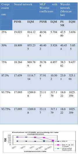
The performances of the MLP model using wavelet coefficients are near or intermediate between those of wavelet model and those of the MLP classic one. These results show a good behaviour of the MLP model using the wavelet coefficients compared to the wavelet network. The following
[image:6.612.305.573.157.685.2]plots present the evolution of the performances in term of EQM and PSNR according to the compression rate of the three analysed models.[7]
Table 1
Compr ession rate
Neural network MLP with Wavelet coefficients
Wavelet network (Mexican hat)
PSNR EQM PSNR EQM PS NR
EQM
25% 19.023 814.12 1
40.56 8
5.704 42.5 00
3.656
50% 18.809 855.23 5
40.40 2
5.926 40.45 4
5.85 5
75% 18.264 969.78 9
39.76 9
6.857 38.3 82
9.437
87.5% 17.659 1114.7 14
37.91 7
10.50 2
23.0 1
325.1 01
93.75% 17.095 1269.0 8
23.11 7
317.1 79
18.0 22
1025. 359
93.75% 17.095 1269.0 8
23.11 7
317.1 79
18.0 22
[image:6.612.49.273.318.533.2]Evolution of the PSNR according to the compression rate for the three models of network
Figure 5
Evolution of the EQM according to the compression rate for the three models of networks
Figure 6
We can deduce that the wavelet networks are more effective when the compression rate is lower than 75%, but less effective when this rate is beyond this limit.
CONCLUSION
In this paper the use of Multi -Layer Perception Neural Networks for image compression is reviewed. Since acceptable result is not resulted by compression with one network, a new approach is used by changing the Training algorithm of the network with modified LM Method.
The proposed technique is used for image compression. The algorithm is tested on varieties of benchmark images. Even though neural networks have a huge potential we will only get the best of them when they are integrated with computing, AI, fuzzy logic and related subjects. Neural networks are performing successfully where other methods do not, recognizing and matching complicated, vague, or incomplete patterns.
FUTURE WORK
Artificial Neural Networks is currently a hot research area in image processing and it is believed that they will receive extensive application to various fields in the next few years. In contrast with the other technologies, neural networks can be used in every field such as medicine, marketing, industrial process control etc. This makes our application flexible and can be extended to any field of interest. Integrated with the other fields like Artificial intelligence, fuzzy logic neural networks have a huge potential to perform. Neural networks have been applied in solving a wide variety of problems. It is an emerging and fast growing field and there is a huge scope for research and development.
REFERENCES
[1] R. P. Lippmann, “An introduction to computing with neural network”, IEEE ASSP mag., pp. 36-54, 1987.
[2] M.M. Polycarpou, P. A. Ioannou, “Learning and Convergence Analysis of Neural Type Structured Networks”,
IEEE Transactions on Neural Network, Vol 2, Jan 1992, pp.39-50.
[3] K. R Rao, P. Yip, Discrete Cosine Transform Algorithms, Advantages, Applications, Academic Press, 1990
[4] Rao, P.V. Madhusudana, S.Nachiketh,S.S.Keerthi, K.
“image compression using artificial neural network”.EEE,
ICMLC 2010, PP: 121-124.
[5] Dutta, D.P.; Choudhury, S.D.; Hussain, M.A.; Majumder,
S.; ”Digital image compression using neural network” .IEEE,
international Conference on Advances in Computing, Control, Telecommunication Technologies, 2009. ACT '09.
[6] N.M.Rahim, T.Yahagi, “Image Compression by new sub -image bloc Classification techniques using Neural Networks”, IEICE Trans. On Fundamentals, Vol. E83-A, No.10, pp 2040-2043, 2000.