How many replicates of arrays are required to detect gene expression changes in microarray experiments? A mixture model approach

comment

reviews

reports

deposited research

interactions

information

refereed research

Research

How many replicates of arrays are required to detect gene

expression changes in microarray experiments? A mixture

model approach

Wei Pan*, Jizhen Lin

†

_{and Chap T Le*}

Addresses: *Division of Biostatistics, School of Public Health, University of Minnesota, 420 Delaware Street, Minneapolis, MN 55455-0378, USA. †_{Department of Otolaryngology, School of Medicine, University of Minnesota, Minneapolis, MN 55455, USA.}

Correspondence: Wei Pan. E-mail: [email protected]

Abstract

Background:It has been recognized that replicates of arrays (or spots) may be necessary for reliably detecting differentially expressed genes in microarray experiments. However, the often-asked question of how many replicates are required has barely been addressed in the literature. In general, the answer depends on several factors: a given magnitude of expression change, a desired statistical power (that is, probability) to detect it, a specified Type I error rate, and the statistical method being used to detect the change. Here, we discuss how to calculate the number of replicates in the context of applying a nonparametric statistical method, the normal mixture model approach, to detect changes in gene expression.

Results:The methodology is applied to a data set containing expression levels of 1,176 genes in rats with and without pneumococcal middle-ear infection. We illustrate how to calculate the power functions for 2, 4, 6 and 8 replicates.

Conclusions:The proposed method is potentially useful in designing microarray experiments to discover differentially expressed genes. The same idea can be applied to other statistical methods. Published: 22 April 2002

GenomeBiology2002, 3(5):research0022.1–0022.10

The electronic version of this article is the complete one and can be found online at http://genomebiology.com/2002/3/5/research/0022 © 2002 Pan et al., licensee BioMed Central Ltd

(Print ISSN 1465-6906; Online ISSN 1465-6914)

Received: 27 December 2001 Revised: 15 February 2002 Accepted: 11 March 2002

Background

Microarrays are used to measure the (relative) expression levels of thousands of genes (or expressed sequence tags). A comparison of gene expression in cells or tissues from two conditions may provide useful information on important biological processes or functions [1,2]. The challenge now is how to detect those genuine changes from noisy data. It is now known that simply using fold changes, as in the earlier days, is unreliable and inefficient [3,4]. More sophisticated statistical methods are called for. Many proposals have appeared in the literature [3-10]. In particular, it has been noticed that it may be necessary to design an experiment that uses multiple arrays (or multiple spots on each array) containing multiple measurements for each gene under each

does not depend on the normality assumption, the problem is that under non-normal situations the t-test may be too conservative, and hence, as with the Wilcoxon test, may have too low power, especially when the sample size is small, which is the case for most microarray experiments. These points have been verified in two case studies using real data [8,12]. In a class of nonparametric approaches [5,9,10], a version of the two-sample t-statistic is used but its null dis-tribution is estimated nonparametrically, rather than directly assumed to be a t-distribution. In addition, some earlier studies have suggested that the variability of gene expression may be related to the mean expression [3,4,6]. Therefore, it implies that the t-statistic being used should be based on unequal variances for the two samples.

An important and natural question often asked by biologists is how many replicates are required. For microarray experi-ments, unlike many other experimental contexts, this issue has rarely been discussed in the literature. To our knowledge, the only exception is the work by Black and Doerge [13], which, however, is for the situation where parametric statisti-cal methods are applied to detect expression changes. In this paper, we discuss the problem when a nonparametric method, the normal mixture model approach [10], is used to detect differential expression. But to facilitate calculations of sample size, the formulation is slightly changed from their original one. Nonparametric methods of microarray data analysis have been pioneered by Efron and Tibshirani and co-workers [5,9]. They take advantage of the presence of replicates and thus can impose much weaker modeling assumptions. For instance, the parametric methods of Black and Doerge [13] depend on the assumption on the log-normal or gamma distribution of gene-expression levels, whereas the mixture model approach does not have such a distributional assumption and directly estimates distributions related to random errors. Note that modeling the distribution of random errors has advantages over direct modeling of expression levels, and is a common practice in applied statis-tics. For example, gene-expression levels may be correlated (for example, as a result of coexpression of some genes) whereas random errors can be more reasonably assumed to be independent. This is similar to modeling longitudinal data using a linear mixed-effects model [14]: the responses from each subject (corresponding to a group of coregulated genes here) are in general correlated, but the measurement errors from the same subject can be considered to be independent after incorporating a random-subject effect in the model. Note that the random effect will be canceled out from the

t-statistic for each gene. Our proposal here also shows an attractive feature of the mixture model approach, as com-pared to the other two nonparametric approaches [5,9], because it is still unclear how the sample size/power calcula-tion can be done in the other two approaches.

The problem of calculating the number of replicates required in a microarray experiment is similar to that of sample

size/power calculations in clinical trials and other experi-ment designs; the (to-be-determined) sample size in microarray experiments refers to the number of replicates, whereas the number of genes is not an issue here. As usual, we assume that the replicates are (approximately) indepen-dent with each other, whether they are drawn from the same individual or multiple individuals. In general, the required sample size depends on several factors: the true magnitude of the change of gene expression (say, d), the desired statisti-cal power (that is, probability) () to detect the change, and the specified Type I error rate (). The problem of how to calculate the number of replicates for any given triplet (d, ,

) is equivalent to that of how the power depends on the pair (d, ) and the number of replicates, which we consider in the paper.

The proposed method is not restricted to any specific microarray technology. From now on, the expression level can refer to a summary measure of relative red-to-green-channel intensities in a fluorescence-labeled cDNA array, a radioactive intensity of a radiolabeled cDNA array (as used in the example later), or a summary difference of the perfect match (PM) and mismatch (MM) scores from an oligo-nucleotide array. The gene-expression levels may have been suitably preprocessed, including dimension reduction, data normalization and data transformation [5,15-18].

Results and discussion

A statistical model

We consider a generic situation that, for each gene i, I = 1,2,...,N, we have (relative) expression levels X1i,..., Xmi from m microarrays under condition 1, and Y_1i,..., Y_mifrom marrays under condition 2. We need to assume that m is an even integer. A general statistical model is assumed for gene expression data:

X_ji= ␮_(1),i+ ⑀_ji, Y_li= ␮_(2),i+ e_li,

where (1),i and (2),iare the mean expression levels for gene

i under the two conditions respectively, and _ji and e_li are independent random errors with means and variances

E(⑀_ji) = E(e_li) = 0, Var(⑀_ji) = ␴2

(1),i, Var(eli) = ␴(2),2 i,

for any j = 1,..., m, l = 1,..., mand i = 1,..., N. It is assumed that random errors _ji/_(1),iand e_li/2

(1),iare randomly taken respectively from one of two (not necessarily equal) distribu-tions that are symmetric about their mean 0. Note that the above assumption on the distributions of random errors, not on that of gene expression levels (that is, X_jiand Y_li), is often reasonable, and similar assumptions are common in other statistical applications. In addition, we do not assume that the expression levels of all the genes have an equal variance, because some previous studies [3,4,6] have found that the variance 2

comment

reviews

reports

deposited research

interactions

information

refereed research

depend on the mean expression _(c),i. Also, we do not even need to assume that 2

(1),i= 2(2),iunless (1),i= (2),i.

A goal is to detect all genes with _{(1),i (2),i}. This can be accomplished through statistical hypothesis testing.

A test statistic

To test the null hypothesis H0: (1),i= (2),i, we use a t-type test statistic or score

m

j=1 Xji/m

m

j=1 Yji/m ␮(1),i ␮(2),i

Zi = ——————— - ——————— = ——— - ——— +

␴(1),i ␴(2),i ␴(1),i ␴(2),i

m

j=1 ⑀ji

n l=1 eli

———— - ————— . (1)

m␴_(1),i m␴_(2),i

Note that the mean and variance of Z_iare

␮(1),i ␮(2),i 2

E(Z_i) = ——— - ————, Var (Z_i) = —— , ␴(1),i ␴(2),i m

whereas the mean E(Z_i) = 0 under H₀. Hence, it can be seen that a large absolute value of Z_i, |Z_i|, gives evidence against

H₀. As the number of arrays (that is, m) increases, the vari-ance of the test statistic Z_idecreases. Hence, it is possible to reject H₀(that is, detect differential expression for gene i) with any E(Z_i) 0 if mis large enough. In other words, if the Type I error rate and other parameters are fixed, then the statistical power of the test will increase as mincreases. This is the key point that motivates the discussion on sample size calculations.

To determine the cut-off point for |Z_i| to reject H₀, we need to know or estimate the distribution of Z_iunder H₀, the null distribution f₀. In a parametric approach, based on some full distributional assumptions for X_jiand Y_ji, one may derive the null distribution f0, such as in a two-sample t-test. However,

the validity of such a parametric method critically depends on the correctness of assumed distributions, which of course is not guaranteed. Here, we consider a nonparametric approach: a finite normal mixture model is used to estimate

f₀ nonparametrically.

Estimating the null distribution

There may be various ways to estimate the null distribution

f₀. For instance, using expression levels of some housekeep-ing genes that are known to have non-differential expres-sion, one can construct their Z_iscores and then estimate f₀

using the obtained Z_iscores. In practice, however, there may be only a small number of or no housekeeping genes in a given experiment. Here, following the basic idea in a class of nonparametric methods [5,9,10], we construct a null score z_i

for each gene and then use these null scores to estimate f0

nonparametrically. The null score is constructed from the same observed gene expression data as used in Z_i:

X_1i - X_2i + … + X_m-1,i- X_m,i Y_1i - Y_2i + … + Y_m-1,i- Y_m,i z_i= ————————————————— + ————————————————

m␴_(1),i m␴_(2),i

⑀1i - ⑀2i + … + ⑀m-1,i- ⑀m,i e1i - e2i + … + em-1,i- em,i

= ——————————————— + ———————————————— . (2)

m␴_(1),i m␴_(2),i

Under the assumption that _jiand e_jihave symmetric distrib-utions, then _jiand -_jihave the same distribution, and e_ji

and -e_jihave the same distribution. Thus, by comparing the form of z_iwith that of Z_i, we know that the distribution of z_i

is exactly f0, the null distribution for Zi(under H0). Note that

under H₀, _(1),i = _(2),i, and hence _(1),i = _(2),I (since we assume that _(c),ionly depends on _(c),i), then

⑀1i + ⑀2i + … + ⑀m-1,i+ ⑀m,i e1i + e2i + … + em-1,i+ em,i

Z_i= ———————————————— + ————————————————— .

m␴_(1),i m␴_(2),i

Thus ziand Zihave the same distribution f0under H0. We

use all z_ivalues across all genes to estimate f₀.

In practice, _(c),i(for c = 1, 2) are unknown, and can be esti-mated using the sample standard deviations (SDs) s_(c),i. Although the sample SD s_(c),iis asymptotically unbiased, if m

and nare small, s_(c),imay not be stable, and some modifica-tions may be necessary. In any case, substituting _(c),iby any suitable estimates, we can calculate the scores zivalues and

Z_ivalues, on the basis of which we can estimate f₀ and f

respectively. By comparing f₀ and f, we can gain insight about genes with altered expression (that is, _(1),i(2),i).

We assume that all the z_ivalues for i = 1,..., Nare a random sample from f₀; thus we can use the observed z_ivalues to estimate f₀. Pan et al. [10] proposed estimating f₀using a finite normal mixture model [19]. Specifically, it is assumed that

g₀

f₀ (z; g0) =

r (z;ar, Vr), r=1

where (z; a_r, V_r) denotes the density function of a normal distribution N(ar, Vr) with mean arand variance Vr, and r values are mixing proportions. _g0represents all unknown parameters {_r, a_r, V_r) : r = 1,...g₀} in a g₀-component mixture model. Among others, a normal mixture is essen-tially nonparametric and flexible, and easy to use with stable tail probabilities.

number of components can be selected adaptively using the Akaike Information Criterion (AIC) [22] or the Bayesian Information Criterion (BIC) [23]. In using the AIC or BIC, one first fits a series of models with various values of g₀, then picks up the g₀ corresponding to the first local minimum of AIC or BIC [24]. Some empirical studies seem to favor the use of BIC [24].

Determining the cut-off point

Once we obtain an estimate of the null distribution f₀, we can determine the cut-off point of the rejection region for testing

H₀. In general, as for a two-sample test, the rejection region can be selected in the tails of f₀ because, under the null hypothesis, Z_ishould be close to the center of f₀, whereas if there is differential expression for gene i, Z_iis likely to be in one of the two tails of f0. The specific choice may depend on

the goal of the analysis. For example, if we are only inter-ested in detecting upregulated genes, we can choose the rejection region at the right-tail of f₀. Our proposed method works for any specified way of determining the rejection region. As f₀ should be symmetric about its mean 0, and often we are interested in both up- and downregulated genes, we propose to take the rejection region at the two tails of f0, {z : f0(z) < C}, where the constant C > 0 is the cut-off

point and depends on the specified (gene-specific) Type I error rate . As usual, C > 0 is chosen such that the rejec-tion rate under H₀is exactly :

= Pr (Z< -Cor Z> Cf₀)

=

-C

-⬁ f0(z)dz +

⬁

C f0(z)dz (3)

g₀

=

_r[(-C;a_r,V_r) + 1 - (C;a_r,V_r)]. r=1

where (.; a, V) is the corresponding cumulative distribu-tion funcdistribu-tion for (.; a, V). Using a numerical algorithm, such as the bisection method [25], we can solve the above equation to obtain Cfor any given .

For microarray data, because we are testing H₀ for each gene, the multiple test problem arises and some control on it is necessary. Usually we can use Bonferroni’s method. For instance, if we want to maintain the genome-wide Type I error rate at the usual 5% level, then the Bonferroni-adjusted gene-specific (that is, test-specific) Type I error rate is

= 0.05/N, where Nis the total number of genes to be tested.

Once Cis determined, we can calculate the power as a func-tion of d, the magnitude of the expression change targeted to be detected. Note that

(1),i (2),i

d= ——— - ———

(1),i (2),i

is the difference of the coefficients of variation under the two conditions. If _(1),i= _(2),i, dcan be interpreted as the change of the mean expression levels from condition 1 to condition 2. Otherwise, it can be regarded as the difference of (varia-tion) standardized mean expression levels. Specifically, we have the power function

(d,) = Pr(Z- d< -Cor Z- d > Cf0)

=

d-C

⬁ f0(z)dz +

⬁

d+C f0(z)dz (4)

g₀

=

_r[(d-C;a_r,V_r) + 1 - (d+C;a_r,V_r)]. r=1

Unsurprisingly, we can see that (d, ) will increase as |d| increases. The effects of having more replicates will reduce the variability of f₀, leading to larger (d, ) for any given d.

Calculation of replicate numbers

Now we describe how to calculate replicate numbers based on some pilot data taken from earlier studies. We use z_{m, i}to explicitly denote the ziscores in (2) with mreplicates. Based on the data we can estimate the density function f_0,m(z;_g0) of z_m,ivalues as a normal mixture

g₀

f0,m(z; g0) =

r (z;ar,Vr). (5) r

From now on, we treat f_{0, m}as known in Equation (5).

With estimated f_0,m, we want to estimate the density function

f_0,mkfor z_mk,i, the z_iscores based on mkreplicates (with k >1). If we can have an estimate of f_{0, mk}, then we can obtain the corresponding power function (d, ) for mkreplicates in the same way as described earlier for mreplicates. Of course, we assume that our pilot data are drawn from only m arrays under each of the two experimental conditions, and thus we do not observe any zmk,i based on mkarrays. However, we show next that it is possible to generate z_mk,ivalues from z_m,i

values. Note that we can draw random realizations of z_m,i

from the estimated f_0,m(see Pan et al. [10] or the example below). Suppose z_{m, i}(j)_{values (for j = 1,2,..., k) are k}

indepen-dent realizations of z_m,i, then it is easy to show that

k

zmk,i=

z

(j)

m,i/k (6)

j=1

have the distribution f_0,mk. Thus, the density function for

z_mk,ivalues is

g_{0 k k}

f_0,mk(z; g0) =

r1…rk (z;

arj/k,

Vrj/k

2_{). (7)}

For example, if we triple the number of replicates, the result-ing density function is

g₀

f_0,3m(z; g0) =

r1r2r3 (z; (ar1+ar2+ar3)/3, (Vr1+

r1,r2,r3=1

V_r2+V_r3)/9).

The number of components of f_0,mk may be too large. For example, if the number of components is g₀ = 3 for m = n = 2, the corresponding numbers of components for m = n = 4,

m=n = 6 and m = n = 8 are, respectively, g₀2 _{= 9, g}

03 = 27 and g₀4_{= 81. In fact, some of these components may be very similar}

or have a negligible role, hence the form of f_0,mkmay be simpli-fied. In the extreme situation, as mk , by the Central Limit Theorem, the mixture model will reduce to a single-component normal distribution. Hence, we propose a simulation-based method to select a more parsimonious model for f_0,mk.

On the basis of the mixture model f_0,min Equation (5), we can generate a random sample of z_m,i(j) _{values [10], from}

which we can calculate z_mk,ivalues using Equation (6). Using

z_mk,ivalues we can fit a normal mixture model for f_0,mk. As we shall show later, we find such a fitted mixture model often contains a smaller number of components than gk

0, as

dictated in Equation (7), leading to a simplified form of f_0,mk.

Summary of the proposed method

In summary, our proposed method of calculating the required replicate number works in the following steps.

Step 1. Suppose that we have pilot gene expression data Xji and Y_jifrom marrays under each condition. Use formula (2) to calculate the scores z_i,m.

Step 2. Use z_i,mand the normal mixture model (5) to esti-mate f_0,m.

Step 3. For a specified Type I error rate , determine the cut-off point C for the rejection region using formula (3), in which f₀is replaced with the estimated f_0,m.

Step 4. For any specified d, calculate the power function

(d,) using formula (4), in which f₀is replaced with the estimated f_0,m.

Step 5. For any given k >1, use formula (7) or (6) to estimate

f0,mk.

Step 6. For a specified Type I error rate , determine the cut-off point Cfor the rejection region using formula (3), in which f₀is replaced with the estimated f_0,mk.

Step 7. For any specified d, calculate the power function

(d,) using formulae (4), in which f₀is replaced with the estimated f0,mk.

Step 8. Repeat Steps 5 to 7 until all k >1 of interest have been tried.

After the power functions for many possible mkreplicates have been obtained, we can determine an appropriate number of replicates by considering all the factors involved, the desired power and Type I error rate, the targeted expres-sion changes and other experimental constraints.

An example

To understand the pathogenesis of otitis media, a study was conducted to identify genes involved in response to pneu-mococcal middle-ear infection and to study their roles in otitis media. Radioactively labeled DNA microarrays were applied to the mRNA analysis of 1,176 genes in middle-ear mucosa of rats with and without subacute pneumococcal middle-ear infection [26]. The data are available for the control group and for the pneumococcal middle-ear infec-tion group. A more detailed descripinfec-tion of how the data were collected and their public availability was provided in Pan et al. [26]. For the purpose of sample size calculations and to mimic many practical situations with only a small number of replicates, we only use m = n = 2 arrays from each group. We first take a natural logarithm transforma-tion for all the observed gene-expression levels (that is, radioactive intensities) so that the resulting distributions are less skewed (which will reduce the number of compo-nents of a fitted mixture model). Then, for each microarray, we standardize the transformed gene-expression levels by subtracting their median.

Because of the small m = 2, the sample SDs may not be stable. One way is to add a small constant as suggested by Efron et al. [5]. Here we follow the idea of Lin et al. [27] and use a loess smoother [28] to nonparametrically model the sample SDs in terms of the mean expression levels (Figure 1). Then we plug in the smoothed SD to calculate z_2,i. Note that an alternative use of SD or its modification in cal-culating z_2,ivalues will not change the basic idea and the fol-lowing steps in sample size calculations.

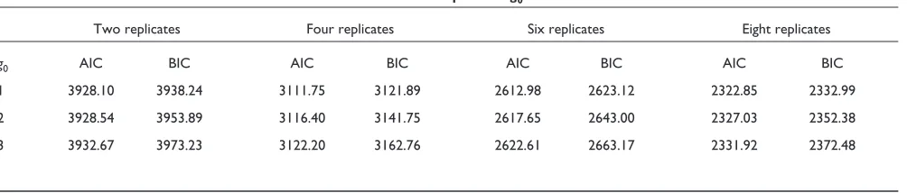
We fitted three mixture models for f_0,2 with g₀ranging from 1 to 3. Table 1 summarizes the model-fitting results. g₀ = 1 was selected as both AIC and BIC achieve their minima there. So the fitted f₀is a normal distribution, N(-0.0013, 0.1278). However, for the purposes of general illustration, we choose g₀ = 2 as the fitted model:

f_0,2(z) = 0.76 (z; -0.0415, 1.3117) + 0.24 (z; 0.0700, 2.6970).

Figure 2a presents the histogram of zivalues and the fitted f0

with g0 = 1 and 2. There is not much difference between the

two fitted f0,2, both of which fit the data well. In particular, f0,2does not look like a t-distribution with small degrees of

freedom, as predicted from the t-test.

comment

reviews

reports

deposited research

interactions

information

A realization of z_2,i can be simulated in the following two steps. First, we draw a random number p_ifrom {1, 2} with probability 0.76 and 0.24 respectively. Second, if the drawn

p_i = 1, z_i is randomly drawn from a normal distribution (z; -0.0415, 1.3117); otherwise, it is drawn from (z; 0.0700, 2.6970). From the generated z2,ivalues, follow-ing expression (6) we generated three simulated data sets:

z_2k,ivalues, I= 1,..., 1,176 for k = 2, 3 and 4. Then a normal mixture model was fitted to each data set. From Table 1, it can be seen that a single-component normal distribution was selected in each case. In Figure 2, each of the fitted normal distributions, N(-0.0494, 0.8226), N(-0.0644, 0.5383) and N(-0.0438, 0.4206), is compared with its theo-retically derived mixture model in Equation (7); they are all very close. Here we see that using simulated data to fit a mixture model results in a much-simplified model. For example, for k = 4, it is a fitted single-component model

versus a 24 _{= 16-component model in Equation (7). Note}

that, as predicted, all the means of the fitted models are all essentially 0, and their variances decrease as kincreases.

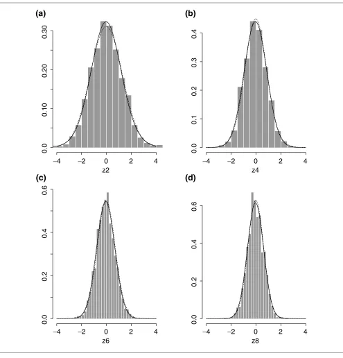
If we want to have only one expected false-positive result from testing each of 1,176 non-differentially expressed genes, the gene-specific (or test-specific) Type I error rate is

[image:6.609.59.556.87.323.2]

= 1/1176 = 0.09%. Using formula (3) and fitted-mixture model f_0,2k, the cut-off points Care determined. Then the power functions (d, ) are drawn in Figure 3, which may help make a decision on the required number of replicates. For instance, if we want to detect an expression change d = 3 with probability at least 80% and with =0.09%, then six replicates are needed. Also, with just two replicates, the power to detect a change as high as 4 is very low, smaller than 30%. Note that the choice of dmay depend on some prior knowledge. For instance, based on the pilot data, we

Table 1

AIC and BIC for fitted mixture models with various number of components g₀

Two replicates Four replicates Six replicates Eight replicates

g₀ AIC BIC AIC BIC AIC BIC AIC BIC

1 3928.10 3938.24 3111.75 3121.89 2612.98 2623.12 2322.85 2332.99

2 3928.54 3953.89 3116.40 3141.75 2617.65 2643.00 2327.03 2352.38

[image:6.609.57.559.636.743.2]

3 3932.67 3973.23 3122.20 3162.76 2622.61 2663.17 2331.92 2372.48

Figure 1

Sample standard deviations of expression levels and their loess smoothers as a function of the average expression levels for the two conditions respectively.

X

0

2

4

6

8

10

0.0

0.05

0.15

0.25

Y

0

2

4

6

8

0.0

0.05

0.15

SD

SD

can estimate the d values for some selected genes (with the sample means and sample SDs substituting the true means and SDs in the formula for d), from which one can determine a range of dvalues of interest.

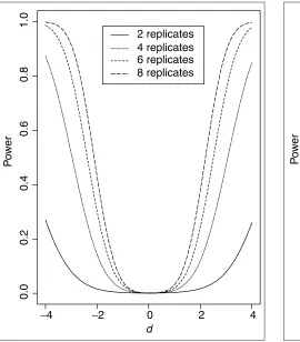
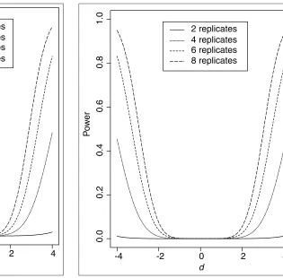
Figures 4-6 give the results for testing N = 1,000, 5,000 and 10,000 genes, respectively, while controlling the genome-wide

Type I error rate at the usual 5% level. It can be seen that as

N increases, we also need a larger number of arrays to maintain the power of the statistical test when other para-meters are fixed. For instance, for N = 10,000 (Figure 6), even eight replicates cannot detect a change as large as

d= 3 with 80% power, but six replicates can detect a change d = 4 with 80% power.

comment

reviews

reports

deposited research

interactions

information

[image:7.609.59.554.84.600.2]

refereed research

Figure 2

Histograms and estimated distribution density functions. (a-d)Two, four, six and eight replicates (z2 - z8), respectively. In (a), the solid and dotted lines are the fitted one- and two-component mixtures. In (b-d), the solid and dotted lines are the fitted and the theoretically derived mixtures.

−

4

−

2

0

2

4

0.0

0.10

0.20

0.30

z2

(a)

−

4

−

2

0

2

4

0.0

0.1

0.2

0.3

0.4

z4

(b)

−

4

−

2

0

2

4

0.0

0.2

0.4

0.6

z6

(c)

−

4

−

2

0

2

4

0.0

0.2

0.4

0.6

z8

Conclusions

We have described a method for calculating the number of replicates in microarray experiments. This method is designed for the situation where the mixture approach is going to be taken to analyze the data. Note that any method for sample size/power calculations has to depend on a spe-cific statistical test to be used in data analysis; this explains why there is a huge literature on the topic for clinical trials. However, because of the close relation between the mixture approach and the other two recently proposed nonparamet-ric approaches - the empinonparamet-rical Bayes method [5] and the sta-tistical analysis of microarray (SAM) method [9] - our proposed method can be also applied to provide some useful guideline for designing microarray experiments even when one of the latter two approaches (or other approaches) is planned to be used for data analysis in a later stage. For instance, even though the null distribution f₀is estimated using the null scores z_iin our proposal, there may be alterna-tive ways of estimating f₀, such as using an alternative non-parametric method (for example, kernel or local likelihood), rather than the finite normal mixture model, to estimate f₀, or using the test statistics, Z_i, of a large number of house-keeping genes to estimate f0. Some modifications to the test

statistic Z_iand the null statistic z_iare also possible, especially when we consider differential gene expression across more than two conditions. These are all interesting topics we are investigating now.

In most sample size/power calculations, some pilot data are needed to provide reasonable estimates of some parameters needed for subsequent calculations. An alternative is to obtain reasonable estimates from other similar studies in the literature. However, because of the rapid development of microarray technology, the latter is not likely and we expect a researcher will have to do his or her own pilot study. This was the situation we considered in the example. A particular chal-lenge is how to obtain good estimates of the variances of gene expression levels from a small number of replicates. In our example, we considered a nonparametric method to smooth sample variances. Some alternative smoothing methods have also appeared in the literature. But it is not clear which one is the most desirable. This is a topic for future study.

[image:8.609.308.554.85.395.2]

The proposed method is straightforward to statisticians and can be implemented in many existing statistical packages. Our sample S-Plus program and data are available at [29].

Figure 3

Power (d, ) as a function of the magnitude of expression changes d and the number of replicates, with the gene-specific Type I error rate = 0.09% for the middle-ear data.

d

Po

w

e

r

−

4

−

2

0

2

4

0.0

0.2

0.4

0.6

0.8

1.0

[image:8.609.58.328.86.394.2]

2 replicates

4 replicates

6 replicates

8 replicates

Figure 4

Power (d, ) as a function of the magnitude of expression changes d and the number of replicates, with the gene-specific Type I error rate = 0.05/1,000 for the middle-ear data.

d

Po

w

e

r

−

4

−

2

0

2

4

0.0

0.2

0.4

0.6

0.8

1.0

Acknowledgements

This research was partially supported by NIH.

References

1. Brown P, Botstein D: Exploring the new world of the genome with DNA microarrays.Nat Genet 1999, 21(Suppl):33-37. 2. Lander ES: Array of hope.Nat Genet1999, 21(Suppl):3-4. 3. Chen Y, Dougherty ER, Bittner ML: Ratio-based decisions and

the quantitative analysis of cDNA microarray images. J Biomed Optics1997, 2:364-367.

4. Newton MA, Kendziorski CM, Richmond CS, Blattner FR, Tsui KW:

On differential variability of expression ratios: improving statistical inference about gene expression changes from microarray data.J Comput Biol 2001, 8:37-52.

5. Efron B, Tibshirani R, Goss V, Chu G: Microarrays and their use in a comparative experiment.Technical Report, Department of Statistics, Stanford University, 2000.

[http://www-stat.stanford.edu/~tibs/research.html].

6. Ideker T, Thorsson V, Siehel AF, Hood LE: Testing for differen-tially-expressed genes by maximum likelihood analysis of microarray data.J Comput Biol2000, 7:805-817.

7. Li H, Hong F: Cluster-Rasch models for microarray gene expression data.Genome Biol2001, 2(8):research0031.1-0031.13. 8. Thomas JG, Olson JM, Tapscott SJ, Zhao LP: An efficient and

robust statistical modeling approach to discover differen-tially expressed genes using genomic expression profiles.

Genome Res2001, 11:1227-1236.

9. Tusher VG, Tibshirani R, Chu G: Significance analysis of microarrays applied to the ionizing radiation response.Proc Natl Acad Sci USA2001, 98:5116-5121.

10. Pan W, Lin J, Le C: A mixture model approach to detecting differentially expressed genes with microarray data. Techni-cal Report 2001-011, Division of Biostatistics, University of Min-nesota, 2001. [http://www.biostat.umn.edu/cgi-bin/rrs?print+2001]. 11. Lee MLT, Kuo FC, Whitmore GA, Sklar J: Importance of

replica-tion in microarray gene expression studies: statistical methods and evidence from repetitive cDNA hybridiza-tions.Proc Natl Acad Sci USA2000, 97:9834-9839.

12. Pan W: A comparative review of statistical methods for dis-covering differentially expressed genes in replicated microarray experiments.Bioinformatics, in press

. [http://www.biostat.umn.edu/cgi-bin/rrs?print+2001]

13. Black MA, Doerge RW: Calculation of the minimum number of replicate spots required for detection of significant gene expression fold change in microarray experiments.Technical Report, Department of Statistics, Purdue University, 2001. 14. Diggle PJ, Liang KY, Zeger SL: Analysis of Longitudinal Data.Oxford:

Oxford University Press, 1994.

15. Dudoit S, Yang YH, Callow MJ, Speed TP: Statistical methods for identifying differentially expressed genes in replicated cDNA microarray experiments. Technical Report, Statistics Department, University of California at Berkeley, 2000.

[http://www.stat.berkeley.edu/users/terry/zarray/Html/matt.html/. 16. Li C, Wong WH: Model-based analysis of oligonucleotide

arrays: expression index computation and outlier detec-tion.Proc Natl Acad Sci USA2001, 98:31-36.

17. Kerr MK, Martin M, Churchill GA: Analysis of variance for gene expression microarray data.J Comput Biol2000, 7: 819-837.

18. Yang YH, Buckley MJ, Dudoit S and Speed TP: Comparison of methods for image analysis on cDNA microarray data.

comment

reviews

reports

deposited research

interactions

information

[image:9.609.226.541.84.394.2]

refereed research

Figure 5

Power (d, ) as a function of the magnitude of expression changes d and the number of replicates, with the gene-specific Type I error rate = 0.05/5,000 for the middle-ear data.

d

Po

w

e

r

−

4

−

2

0

2

4

0.0

0.2

0.4

0.6

0.8

1.0

2 replicates

4 replicates

6 replicates

8 replicates

Figure 6

Power (d, ) as a function of the magnitude of expression changes d and the number of replicates, with the gene-specific Type I error rate = 0.05/10,000 for the middle ear-data.

d

Po

w

e

r

-4

-2

0

2

4

0.0

0.2

0.4

0.6

0.8

1.0

[image:9.609.55.303.87.396.2]

Technical Report, Statistics Department, University of California at Berkeley, 2000.

[http://www.stat.berkeley.edu/users/terry/zarray/Html/image.html]. 19. Titteringto DM, Smith AFM, Makov UE: Statistical Analysis of Finite

Mixture Distributions.New York: Wiley, 1985.

20. Dempster AP, Laird NM, Rubin DB: Maximum likelihood from incomplete data via the EM algorithm. J Roy Stat Soc Ser B 1977, 39:1-38.

21. McLachlan GL, Basford KE: Mixture Models: Inference and Applications to Clustering.New York: Marcel Dekker, 1988.

22. Akaike H: Information theory and an extension of the maximum likelihood principle.2nd International Symposium on Information Theory. Edited by Petrov BN, Csaki F. Budapest: Akademiai Kiado, 1973; 267-281.

23. Schwartz G: Estimating the dimensions of a model.Annls Statis-tics1978, 6:461-464.

24. Fraley C, Raftery AE: How many clusters? Which clustering methods? - Answers via model-based cluster analysis. Com-puter J1998, 41:578-588.

25. Press WH, Teukolsky SA, Vetterling WT, Flannery BP: Numerical Recipes in C, The Art of Scientific Computing.2nd edn. New York: Cam-bridge University Press, 1992.

26. Pan W, Lin J, Le C: Model-based cluster analysis of microarray gene expression data. Genome Biol 2002, 3(2) :research009.1-research009.8.

27. Lin Y, Nadler ST, Attie AD, Yandell BS: Mining for low-abun-dance transcripts in microarray data. Technical Report, Department of Statistics, University of Wisconsin-Madison, 2001. [http://www.stat.wisc.edu/~yilin/].

28. Cleveland W, Devlin SJ: Locally weighted regression: an approach to regression analysis by local fitting.J Am Stat Assoc 1988; 83:596-610.

29. Statistical analysis of microarray data