An empirical analysis of organized crime,
corruption and economic growth
Rana, MP, Neanidis, KC and Blackbourn, K
http://dx.doi.org/10.1007/s1043601702997
Title
An empirical analysis of organized crime, corruption and economic growth
Authors
Rana, MP, Neanidis, KC and Blackbourn, K
Type
Article
URL
This version is available at: http://usir.salford.ac.uk/id/eprint/45007/
Published Date
2017
USIR is a digital collection of the research output of the University of Salford. Where copyright
permits, full text material held in the repository is made freely available online and can be read,
downloaded and copied for noncommercial private study or research purposes. Please check the
manuscript for any further copyright restrictions.
DOI 10.1007/s10436-017-0299-7
R E S E A R C H A RT I C L E
An empirical analysis of organized crime, corruption
and economic growth
Kyriakos C. Neanidis1 · Maria Paola Rana1 · Keith Blackburn1
Received: 30 March 2017 / Accepted: 29 May 2017 / Published online: 9 June 2017 © The Author(s) 2017. This article is an open access publication
Abstract In a companion study, Blackburn et al. (Econ Theory Bull,2017), we have developed a theoretical framework for studying interactions between organized crime and corruption, with the view of examining the combined effects of these phenomena on economic growth. The analysis therein illustrates that organized crime has a neg-ative effect on growth, but that the magnitude of the effect may be either enhanced or mitigated in the presence of corruption. In this paper we tackle the ambiguity pro-duced by the coexistence of the two illicit activities with an empirical investigation using a panel of Italian regions for the period 1983–2009. We find that organized crime distorts growth less when it coexists with corruption and show our results to be robust to different specifications, measures of organized crime, and estimation techniques.
Keywords Corruption·Economic growth·Italy·Organized crime
JEL Classification C23·K49·O43
1 Introduction
It is well-accepted that criminal organizations typically involve the collusion or direct participation of the public sector in their illegitimate activities. In 1994, the United Nation’s Naples Declaration officially recognized that organized crime has a “cor-rupting influence on fundamental social, economic, and political institutions”, and that it commonly uses “violence, intimidation and corruption to earn profit or control
B
Kyriakos C. Neanidis1 Department of Economics, Centre for Growth and Business Cycle Research,
territories or markets”.1More recently, a survey based on public perceptions of the links between corruption and organized crime conducted byEurobarometer(2006), revealed that more than half of European citizens believe that most of the corruption in their countries is related to organized crime. Even more recently, in 2015, the United Nations have agreed on seventeen new global Sustainable Development Goals as part of their 2030 Agenda.2Amongst them, Goal 16: Peace, Justice and Strong Institu-tions, acknowledges the links between these two illicit phenomena and highlights the importance of combating them jointly.
It is not difficult to understand that criminal syndicates strongly depend on, and encourage, corruption in order to carry out their activities with reduced risk of detection and prosecution. Such activities are likely to be more successful with the compliance of law enforcement officers who are willing to accept bribes in return for various favors. Due to this relationship, organized crime can foster corruption at all levels of public office. This is evidenced in a report by Center for the Study of Democ-racy(2010) which focuses on the links between organized crime and corruption in 27 European Member States. The report reveals that criminal organizations have strong links and in-roads to police forces, using their influence to gain access to undisclosed information on investigations, to guarantee endurance of operations, and to develop and maintain monopolies in local markets. The report also emphasizes the signif-icant relationship between organized crime and political corruption (ranging from government ministers and other high-level politicians, to local mayors and city coun-cilors).
The general conclusion of most observers and practitioners is that organized crime flourishes most when the functioning of society’s public institutions is undermined by corruption. Evidence of this can be found in several empirical studies cover-ing various countries in different regions of the world and at different stages of socio-economic development: examples includeMazzitelli(2007) for West Africa, Sergi and Qerimi(2007) for South-East Europe, andBuscaglia and Van Dijk(2003) for a more global sample of territories. Theoretical work on the issue has focused largely on the role of corruption in influencing and compromising strategies to combat organized crime. Becker and Stigler (1974) were the first to point out that the payment of bribes by criminals to law enforcers can weaken the threat of prosecution for criminal activity, suggesting that deterring such activity could be strengthened by remunerating public enforcers sufficiently well and/or pay-ing private enforcers accordpay-ing to performance. In subsequent work, Bowles and Garoupa (1997) showed why the standard prescription of imposing the maximum fine on criminals may not be optimal when there is complicity between the crimi-nal and arresting officer at the expense of the police department.Chang et al.(2000) introduce subjective psychic costs of corruption (moral shame and social stigma), demonstrating how social norms may create conditions under which an increase in fines for criminal activity are counter-productive. Along related lines, Kugler et al.
1 UN GA Resolution 49/159 Naples Political Declaration and Global Action against Organized
Transna-tional Crime (23/121994); UN GA Resolution 1996/27 Implementation of the Naples Political Declaration and Global Action Plan against Organized Transnational Crime (24/07/1996).
(2003) identify circumstances where strategic complementarities between corrup-tion and organized crime mean that tougher sanccorrup-tions on crime produce higher rates of crime, whilst Polinsky and Shavell (2001) suggest that sanctions against corruption, rather than sanctions against crime, are optimal in mitigating criminal behavior.
Whilst the foregoing research has yielded valuable insights on the links between corruption and organized crime, there is still considerable room for further investi-gation. A particularly fertile area, which so far has gone undetected, is the extent to which this link may have an influence on overall economic performance. An attempt in this direction has been made by Blackburn et al.(2017) in a companion study (henceforth BNR), who took a step beyond the partial equilibrium analysis of individ-ual decision making towards the relatively unexplored general equilibrium analysis of aggregate growth outcomes. In a series of overlapping generations endogenous growth models, BNR study the interactions between organized crime and corruption, together with the individual and combined effects of these phenomena on economic growth. In this environment, a criminal organization co-exists with law-abiding pro-ductive agents and potentially corrupt law enforcers. The crime syndicate obstructs the economic activities of agents through extortion, and may pay bribes to law enforcers in return for their compliance in this. The first finding of the analysis is that the presence of organized crime on its own reduces economic performance by deterring agents from engaging in growth-promoting ventures. The second finding, and the main contribution of the study, is that this effect may be either exacerbated or mit-igated by the coexistence of both organized crime and corruption. In other words, the analysis gives rise to an ambiguity of the comparative static over the equilibrium growth rate with crime as compared to the growth rate with both crime and corrup-tion.
Prompted by the inconclusive result of BNR, in this paper we conduct a rigor-ous econometric analysis with the aim of resolving the above ambiguity. We carry out an investigation at the cross-regional level for Italy due to the wealth of data on crimes ascribable to organized criminal groups, unavailable at the international level. Importantly, the variety of data on Mafia-related crimes, available for a rather long period, allows us to construct a multiplicity of indexes that proxy for the dif-ferent activities that typically involve organized criminal organizations. Using growth regression analysis for the period 1983–2009, we find strong evidence that the growth-reducing effect of organized crime is less severe in the presence, than the absence, of corruption. We interpret this as evidence that in the presence of criminal activity, corruption ameliorates the negative effects of organized crime on growth. This find-ing lends support to one of the two plausible theoretical possibilities and suggests the joint treatment of the two illegal phenomena in the context of growth analy-sis.
2 Descriptive summary of a model
In this section, we briefly describe the theoretical model developed in BNR and illus-trate its main predictions.3 The general framework used in our theoretical analysis describes a dynamic, endogenously-growing economy populated by heterogeneous agents engaged in different occupations. The engine of growth is capital accumu-lation, and the set of occupations may include both legal and illegal activities. The former consist of the production of output and capital, together with the enforcement of governance. The latter consist of illicit profiteering by private individuals and pub-lic officials. The description of the model proceeds in three stages. In the first stage, we assume an economy free from any malevolent behavior. In the second stage, we introduce such behavior in the form of organized criminal activity, while in the third stage we also add corruption and explore the implications of the coexistence of these two phenomena for economic growth.
In each of the stages, we consider an overlapping generations economy in which there is a constant population of two-period-lived agents. Each generation of agents is divided at birth into two groups of citizens—a unit mass of households (or workers) and a unit mass of firms (or entrepreneurs). The former are suppliers of labor when young and consumers of output when old. The latter are (potential) producers of capital when young, and producers and consumers of output when old. All agents are risk neutral and all markets are competitive.
The key aspect of the model and the driver of economic growth is the mass of entrepreneurs, who have heterogeneous effort costs. The measure of these producers who decide to invest on a project from which capital is produced depends on their perceived effective rate of return, which gives rise to a critical level of required effort above which capital production is undertaken by an entrepreneur. With the key factor in determining growth being the population of capital producers, any aspect of the environment that influences the critical level of effort, also influences the equilibrium growth rate of the economy. In the absence of any illicit behavior, where agents operate under perfect markets and perfect governance, growth depends only on the return from, and cost of, undertaking capital production. As such, growth is higher the greater is the number of entrepreneurs who optimally choose to be producers of capital.
In the second stage, we introduce crime into the model by considering the case in which entrepreneurs are exposed to extortion by an illicit organization, the Mafia. Like all other agents, the Mafia behaves optimally by choosing its racketeering activities so as to maximise its expected payoff. Implicit in the model is a system of law enforcement designed to obstruct and prevent, detect and prosecute, criminal behavior. It is assumed that the law enforcers act with full integrity in executing their crime prevention duties, i.e., they are not corruptible. In this environment, the Mafia extorts a payment from each capital producer due to a threat of personal damage. It is the payment of the extortion that gives rise to a lower critical level of required effort, compared to the absence of Mafia, above which an entrepreneur chooses to engage in capital production. This, in turn, means that organized crime has the effect of deterring capital production by
some entrepreneurs who would have otherwise engaged in this venture. As an outcome, organized crime lowers the equilibrium growth rate compared to an economy without crime since it effectively acts as a tax on the entrepreneurs’ expected returns.
In the third stage, we consider the case in which law enforcers are potentially willing to accept bribes from the Mafia in return for turning a blind eye to the Mafia’s activi-ties. Therefore, a criminal organization co-exists with law-abiding productive agents and potentially corrupt law enforcers. As before, the crime syndicate impedes legiti-mate economic activities through extortion, but now it may also bribe law enforcers. This means that the payment of bribes acts a tax on the criminals’ expected return, which alongside the extortion applied on entrepreneurs, creates an unfavorable busi-ness environment. The outcome is a higher cost of investment for entrepreneurs that reduces their number and, subsequently, economic growth. Both costs of illegal activi-ties on the formal economy-extortion and bribes-show that growth in a badly-governed economy is lower than growth in a well-governed economy.
The main message of the analysis is that an economy performs better when it is free from all crime and corruption than when it is saddled with either or both these. But, is an economy damaged by more or less if crime occurs alone than if crime co-exists with corruption? The analysis provides no definitive answer to this question. Since the ultimate factor in impeding growth is the Mafia’s extortion of capital producers, the question of which type of environment suffers the most damage is effectively a question of which type of environment suffers the most racketeering. This reduces to a comparison between the expected extortion payment in the presence of crime alone with the extortion payment in the presence of both crime and corruption. Intuitively, corruption reduces the supply of crimes, but makes crimes that occur more likely to be successful. This makes comparative statics ambiguous on the equilibrium growth rate with organized crime versus the growth rate with both crime and corruption. Thus, the foregoing descriptive analysis shows that the impact of organized crime may be conditional on the presence of corruption, and the direction could go either way— organized crime may be more or less damaging if it co-exists with corruption. It is this ambiguity we tackle next with our empirical investigation.
3 Estimation strategy and techniques
The ambiguous prediction of the theoretical analysis in BNR leaves open the question as to whether the combination of organized crime and corruption is more damaging to an economy than organized crime alone. We now proceed to an empirical investigation of the issue using regional Italian data over a 27 years history in order to shed light to this indefinitive result.4Ideally, one would seek to resolve the issue by first considering an economic entity’s growth performance in the absence of both organized crime and corruption, and then adding each of these factors in turn until both are accounted for simultaneously. In this way, one could assess the growth effect of organized crime both in isolation and in conjunction with corruption. In the absence of this ideal scenario
4 The use of data on Italian regions, rather than at the cross-country level, is primarily driven by the
that has been followed in the theoretical framework, our empirical strategy involves specifying a growth equation that controls for both organized crime and corruption, amongst other variables. This growth equation is directly derived from the growth rate expressions in BNR when only organized crime is present and when it coexists with corruption [see Eqs. (15) and (22) of the model], after log-linearization around the steady state. The major element of this growth regression equation is an interaction term between the two illegal activities, which we use to proxy for the growth effect of organized crime in the presence of corruption.5 It is this interaction term that commands most of our attention: the finding of a positive (negative) coefficient on this term would support the argument that organized crime has a less (more) severe effect on growth when it is accompanied by corruption.6
Given the above, our empirical set-up is represented by the following regression equation,
gi,t =α+β1OCi,t+β2Corri,t+β3(OC×Corr)i,t + m
j=1
γjXj,i t +μi+εi,t,
(1)
where variables are indexed by both region,i, and time period,t. These variables are as follows:gis the growth rate of per capita real GDP;OCis a measure of organized crime;
Corris a measure of corruption;X is a set of standard control variables;μcaptures unobserved time-invariant region-specific effects; andεdenotes a time-varying error term. The crucial component is(OC×Corr), which represents the interaction term
between organized crime and corruption.
The set of controls,X, comprises the usual explanatory variables that are included in growth regressions (e.g.,Barro 1991;Levine and Renelt 1992;Sachs and Warner 1997). These are the log of initial real GDP per capita, the ratio of investment to GDP, the rate of inflation (as measured by the GDP deflator), and the rate of secondary school enrolment. In addition to these baseline variables, we consider an extended group of controls, composed of the rate of population growth, the ratio of trade to GDP, the share of total public spending to GDP, and an indicator of financial development.
Our measure of corruption,Corr, departs from the corruption perception indices that are used most commonly in cross-country empirical work.7 The measure that we employ is the official number of crimes against public administration per 100,000 inhabitants reported to the police and published by the Italian National Institute of Statistics (ISTAT). The crimes that we consider are based on Statutes no. 286 through 294, which include crimes of peculation and embezzlement. Other crimes against
5 The interaction term allows controlling for a key point in the models of BNR, the fact that the existence
of corruption creates selection on the amount of equilibrium criminal activity. Further, the use of interaction terms as proxying for conditional effects in the economic growth process has become popular over the years. See, for example,Ahlin and Pang(2008) andAngeles and Neanidis(2009).
6 In terms of the analysis in BNR, a positive (negative) interaction term would imply thatpis large (small)
relative toβ, in which casegc<gcc(gc>gcc).
7 The most popular of these indices are the Corruption Perception Index (published by Transparency
public administration, such as insulting a public officer (Statute 279) and neglect or refusal of an official duty (Statute 295), are excluded. The same measure has been used byDel Monte and Papagni(2001,2007) in previous empirical analyses of corruption in Italy.8Needless to say, the measure may not give a full picture of corruption, and is likely to underestimate such activity, since it is based only on crimes that are reported.9 Accordingly, the estimated coefficient onCorrmay be viewed as representing a lower bound on the effect of corruption.
As regards our measure of organized crime, OC, we follow the existing liter-ature (e.g.,Caruso 2008;Daniele 2009;Daniele and Marani 2010;Pinotti 2011) by constructing different indices of such crime, based on different combinations of Mafia-related offences, and using these alternatively throughout the analysis.10Our preferred measure, however, is an index (labelled OC Index 5) composed of the sum of official data on five different types of crime that are indicative of the presence of criminal organizations, either by definition or by inference.11The five offences are: (i) crimi-nal association (art. 416 Italian Pecrimi-nal Code), (ii) Mafia crimicrimi-nal association (art. 416 bis Italian Penal Code), (iii) homicides by the Mafia, (iv) extortion, and (v) bomb attacks.12A few comments on these are worth making.
Since 1982, the Italian judicial system has made a clear distinction between criminal association (art. 416) and criminal association of Mafia-type groups (art. 416 bis).13 Common criminal association is defined as “the association of three or more people who are organized in order to commit a plurality of crimes”. The characteristics of this kind of offence are the following: (i) the stability of the agreement amongst members, meaning the existence of an associative connection intended to be continuous through time, even after the crimes have been committed; and (ii) the existence of a programme of delinquency to commit an indeterminate number of crimes.14By contrast, a criminal
8 We thank Erasmo Papagni for kindly sharing the data for the years 1961–2001. Data from 2002–2005
can be found online at the ISTAT website. For the most recent data on corruption (2006–2009), we thank ISTAT officers for the collection and transmission of the data.
9 Moreover, as pointed out byDel Monte and Papagni(2001,2007), the measure could also be affected
by a systematic bias due to differences among regions in reporting crimes. This does not, however, seem to be case. By regressing the statistics on reported crimes of corruption and an index of the length of the judicial processes, the authors do not find any large systematic differences among regions in the proportion of reported and detected crimes to actual ones.
10 The term Mafia is used to include all the main criminal organizations that are present in the different
Italian regions, such as Cosa Nostra in Sicily, Camorra in Campania, N’drangheta in Calabria, and Sacra Corona Unita in Puglia.
11 As pointed out byDaniele and Marani(2010) andLa Spina and Lo Forte(2006), even if one cannot
always distinguish organized crime from non-organized crime, it is possible to identify some types of offence (e.g., fraud, theft and sexual violence) as being uncharacteristic of Mafia-type groups.
12 For all crimes, we use rates per 100,000 inhabitants reported by the police to the judicial authority. These
data are available by ISTAT, Annals of Judicial Statistics.
13 Until 1982, Article 416 of the Italian Penal Code (“associazione a delinquere”) punished in the same
way all groups of three or more people involved in some type of criminal activity. This generic term could not distinguish between small groups of bank-robbers and larger criminal networks with a powerful control over the territory. This changed in 1982 with the introduction of the crime “associazione a delinquere di stampo mafioso” provided by Article 416 bis (Law 646/82).
14 This definition is similar to the one given by the UN Convention against Transnational Organized Crime
association is defined to be of the Mafia-type “when its members use intimidation, awe and silence (omert à) in order to commit crimes, to acquire the control or the management of business activities (i.e., concessions, permissions, public contracts or other public services), to derive profit or advantages for themselves or others, to limit the freedom of exerting the right to vote, and to find votes for themselves or others during the electoral campaign”.15 It is necessary to include both types of criminal associations in the definition of organized crime because often it is difficult to prove the Mafia associations, insofar many crimes that are classified as “simple” criminal association are actually Mafia criminal association.
The ultimate of all crimes, that one often associates with Mafia-type organizations, is homicide. As emphasised byMacDonald(2002), all judicial-based measures of crime are generally subject to under-reporting. This may be especially true for offences com-mitted by criminal cartels, whose use of intimidation and violence can undermine the process and outcome of judicial investigations, particularly in regions where the crime syndicate wields a high degree of power and influence. At the same time, there is evi-dence to suggest that under-reporting tends to be smaller for very serious crimes (e.g., Fajnzylber et al. 2002;Soares 2004), hence the inclusion of Mafia-related homicides in the index of organized crime.
Another felony that is prominently linked with organized crime is extortion. Indeed, this is often regarded as the most typical Mafia offence, being a primary means of obtaining illegal income by preying on businesses. In Italy, the commonly-used term for extortion is thepizzo, meaning the black tax that the Mafia imposes on businesses to fund its various operations. According to the Italian shopkeepers association, Con-fesercenti(2009), “the pizzo ensures the everyday activity of criminal organizations, it increases its domain, it confers more prestige to the clans, and measures the rate of silence in a given area, headquarter, or community”. This is echoed elsewhere in the literature, and it is well-documented that almost all the Mafia families exercise their power over a territory through the racket of extortion (see, for example,Daniele and Marani 2010). AsConfesercenti(2009) also points out, official data on racketeering is often susceptible to the aforementioned problem of under-reporting. Nevertheless, the staggering scale of the offence is transparent for all to see: for example, the year 2009 saw a total of 160,000 commercial activities in various Italian regions (mainly Sicily, Campania, Puglia and Calabria) being subject to extortion, with total revenues estimated to be near 9 billion euros.16
Footnote 14 continued
period of time and acting in concert with the aim of committing one or more serious crimes or offences […] in order to obtain, directly or indirectly, a financial or other material benefit”.
15 The last two activities of Mafia-type organizations were introduced into the Italian penal code in 1992
as part of the measures adopted after the Capaci and Via D’Amelio’s massacres (where the judges Giovanni Falcone and Paolo Borsellino were killed). Additionally, art. 416 bis provides for the confiscation of mafia-owned properties.
16 More precisely, the percentage of shops subject to extortion by mafia-type organizations is as high as
A further crime that is typically attributed to criminal organizations is bomb attacks. For the most part, this form of extreme violence is used to threaten and intimidate businessmen who resist being extorted, or politicians who refuse to collaborate. The obvious distinguishing feature of this offence is its visibility when actually committed. Consequently, official data on bomb attacks is much less prone to the problem of under-reporting, and may be used as additional information on other crimes (extortion, in particular) that are committed with the aid of such violence.17
As mentioned, the sum of the above five Mafia-related offences comprises our base-line index of organized crime (OC Index 5). To test the robustness of our benchmark findings, we also use a variety of other indices which include crimes of arson, serious robberies and kidnappings. Arson is considered for the same reason as bomb attacks, being indicative of extortionary activity (and more general intimidation) on the part of criminal groups. Serious roberries (defined as those committed in banks and post offices) are considered since they typically require a high degree of organization and collaboration amongst a plurality of individuals.18Kidnapping is considered because of the historical record of many Mafia organizations in specializing in this offence, as alluded to in previous studies (e.g.,Ciconte 1992;Pinotti 2011).19
The general prediction of theoretical models, including BNR, is that both organized crime and corruption distort economic growth. If so, then the coefficients β1 and
β2 in (1) would be negative and statistically significant. As indicated earlier, our
primary focus is on the growth effect of organized crime conditional on the presence of corruption. This effect is captured by the coefficientβ3, a positive (negative) value
of which would indicate that organized crime is less (more) damaging to growth in regions where corruption is more pronounced. The low correlation between the two key variables, which ranges from 0.09 to 0.31 depending on the measure of organized crime, allows for sufficient variation to estimate the relationship.
Our estimation methods include OLS, region fixed effects (FE) and dynamic panel techniques (difference-GMM and system-GMM), the latter commonly used in the empirical growth literature. The GMM estimations are the most appropriate since they are based on techniques that control for (i) potential endogeneity of the regres-sors, (ii) region-specific effects, and (iii) heteroskedasticity and autocorrelation within regions.20On the other hand, a difficulty associated with these estimators relates to
Footnote 16 continued
in Palermo. More elegant shops in the city centre pay almost 500–1000 euros in Naples and 750–1000 euros in Palermo. The average monthly pizzo is even higher for supermarkets, which are forced to pay the mafia up to 3000 euros in Naples and up to 5000 euros in Palermo. Construction sites may pay as much as 10,000 euros per month in Palermo.Asmundo and Lisciandra(2008) have estimated that in Sicily, the annual total revenues from extortion in 2009 were higher than 1 billion euros, which corresponds to more than 1.3 percent of regional GDP.
17 Of course, the picture is still incomplete since the mere threat of bomb attacks may preclude the need
for them.
18 Serious robberies are also included in the OC index proposed by ISTAT.
19 According toCiconte(1992), among 620 kidnapping cases that have been registered in Italy in the
period 1969–1989, approximately 200 can be attributed to ‘Ndrangheta and only 8, of more than 400, billions Italian lire that have been paid for kidnapping for extortion have been intercepted.
20 An advantage of these estimators is that they avoid a full specification of the serial correlation and
the choice of the number of lags of the endogenous and predetermined variables. In order to restrict the number of instruments so as not to excessively exceed the number of regions (and thus avoid over fitting of the instrumented variables), we use a lag structure of two to four lags for difference-GMM and two to three lags for system-GMM.21
In both the system- and difference-GMM estimations, we test the validity of the instruments by applying two specification tests. The first isHansen(1982) J-test of over-identifying restrictions which we use to examine the coherency of the instruments. The second isArellano and Bond(1991) test for serial correlation of the disturbances up to second order. This test is important since the presence of serial correlation can cause a bias to both the estimated coefficients and standard errors. The appropriate check relates only to the absence of second-order serial correlation since first-differencing induces first-order serial correlation in the transformed errors.
The system-GMM estimator imposes an additional assumption to be satisfied relative to the difference-GMM estimator. This assumption requires a stationarity restriction on the initial conditions of GDP per capita. In particular, the region fixed effects have to be orthogonal to the lagged level of growth rates. According toBond et al.(2001), this estimator has superior finite sample properties by combining “the standard set of equations in first-differences with suitably lagged levels as instruments, with an additional set of equations in levels with suitably lagged first-differences as instruments.” Empirically, the validity of these additional instruments for the levels equation, which are the most suspect in system-GMM, is tested using a Difference-in-Hansen test that compares the first-differenced GMM and system-GMM results.
4 Data
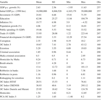
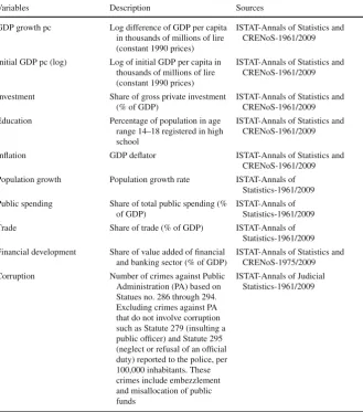
We use a panel of 19 Italian regions for the period 1983–2009.22 Depending on our measure of organized crime, the period considered in different estimations may vary due to data availability.23 Table7in “Data appendix” section provides definitions,
Footnote 20 continued
system-GMM estimator is computed using the finite-sample correction to the two-step covariance matrix derived byWindmeijer(2005) which allows for the estimation of robust standard errors.
21 We use a different lag structure for each estimator so that both estimators end up with similar number of
instruments to assist comparability. In each case we have to collapse the instrument set so that we create one instrument for each variable and lag distance, rather than one for each time period, variable, and lag distance. In large samplescollapsereduces statistical efficiency, but in small samples it can avoid the bias that arises as the number of instruments climbs toward the number of observations (Roodman 2006). We have also experimented with the use of just the second lag as an instrument and the use of fewer variables as being instrumented for (organized crime, corruption and their interaction) instead of collapsing the instruments. In each case the number of instruments greatly exceeds the number of regions, although our findings do not change. For this reason, we do not show these results.
22 We exclude Valle d’Aosta, since it is the smallest and richest region and is usually excluded in the
empirical analysis of Italian regions, being treated as an outlier.
23 For instance, data on homicides by the Mafia, criminal association, extortion, arson and serious robberies
Table 1 Summary statistics
Variable Mean SD Min Max Obs
GDP p.c. growth (%) 2.63 2.56 −3.95 11.63 257 Initial GDP p.c. (1990 lire) 18,900,000 8,068,528 4,165,179 39,000,000 257 Investment (% GDP) 24.81 6.68 15.81 71.55 240
Education 62.06 25.27 11.84 104.79 260
Inflation (%) 19.77 6.98 5.9 −4.52 260
Population growth (%) 4.06 3.67 0.12 16.01 257 Public spending (% GDP) 19.46 5.53 9.62 33.52 200
Trade (% GDP) 33.95 28.08 1.22 223.44 207
Financial development (% GDP) 20.03 3.33 12.29 27.54 140
Corruption 2.35 1.98 0.19 10.2 257
OC Index 5 10.67 7.41 2.78 43.12 160
Extortion 5.29 3.55 0.89 19.03 200
Criminal association 1.85 0.96 0.44 6 200
Mafia criminal association 0.3 0.5 0 2.95 160
Homicides by Mafia 0.24 0.71 0 6.73 200
Bomb attacks 2.37 4.28 0 24 160
Arsons 13.4 12.72 2.02 101.13 200
Robberies in banks 2.34 1.68 0 7.38 160
Robberies in posts 1.16 0.96 0 6.81 160
Kidnapping for extortion 0.24 0.2 0 1.11 200
OC Index ISTAT 20.51 15.53 4 76.61 120
OC Index CRENOS 38.93 40.6 3.19 295.12 200
OC Index Daniele and Marani 25.95 18.62 7.44 124.78 160
Homicides 1.54 1.62 0.21 12.85 257
PCA OC Index 5 1.25 1.65 −1.48 8.2 160
Data on GDP per capita growth, investment, inflation, secondary school enrolment, trade, public spend-ing, financial development and population growth are from CRENOS and the Italian National Institute of Statistics (ISTAT), Annals of Statistics (various years). For these variables, summary statistics are based on average data for the period 1961–2009. Data on crimes are from ISTAT, Annals of Judicial Statistics (various years). The period of time considered for the averages depends on the availability of data (see Table7in “Data Appendix” section for a detailed description of the availability of data)
sources and the exact period availability of the data, whilst Table 1presents some summary statistics. Following the standard approach, we construct 7 non-overlapping 4-year period averages(1983−1986,1987−1990, . . . ,2007−2009)in order to mini-mize business cycles effects. This implies a maximum sample size of 133 observations when we use our baseline measure of organized crime (OC Index 5), though sometimes we end up working with fewer observations due to missing data.24
24 When we use the measure of OC available since 1961, we construct 13 non-overlapping 4-year period
5 Baseline results
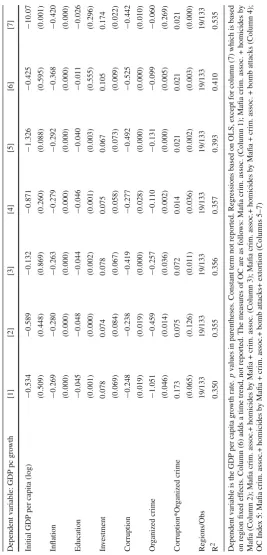
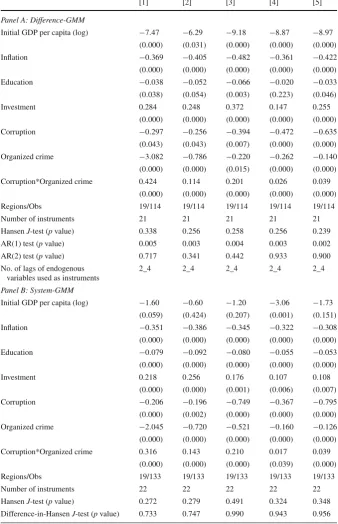
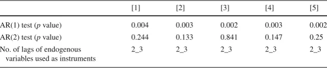
We begin our analysis by estimating Eq. (1) first with OLS and FE and then with difference- and system-GMM to account for the potential endogeneity of all the right-hand-side variables. The OLS and FE results are reported in Table2, while the GMM results appear in Table3(difference-GMM in Panel A and system-GMM in Panel B). Each of the first five columns shows the results for a different measure of organized crime. Column 1 reports the results using the simplest index of organized crime— namely, Mafia criminal association. The subsequent columns give the results based on indices that are constructed by adding, in turn, each of the following types of organized crime: homicides by the Mafia, criminal association, bomb attacks, and extortion. The index used in column 5 (OC Index 5) is the most complete measure and represents our baseline measure of organized crime. Columns 6 and 7 also use this more complete index, but also control for a time trend and region fixed effects, respectively.
With regard to instrumentation, when using GMM techniques, the small number of Italian regions constrains us in keeping the maximum number of lags to four for difference-GMM and to three for system-GMM, in order to maintain the number of instruments at a minimum. Despite this tight restriction, in each case the instruments appear to be valid according toHansen(1982) specification test, whilst theArellano and Bond(1991) test does not reject the null hypothesis of no second-order serial corre-lation, at any acceptable level of significance. Similarly, the Difference-in-Hansen test, focusing on the additional instruments used by the system-GMM estimator, supports the instrument validity.25
Both Tables2and3illustrate the typical findings of growth regressions: there is conditional income convergence, a positive statistically significant effect of invest-ment, and a negative statistically significant effect of inflation.26As found elsewhere in the empirical growth literature, both at the cross-country level (e.g.,Benhabib and Spiegel 1994) and for the case of Italy (e.g.,Di Liberto 2008), the coefficient on edu-cation is estimated to be negative. This result may be due to the specific measure of education that we use to proxy for human capital (secondary school enrolment rates) or due to the distorted structural composition of the Italian labor force and the inefficient allocation of human capital across sectors.
With regard to the variables of most interest to us, our results confirm those of previous studies, showing that the coefficients on corruption and organized crime are negative and statistically significant in all regressions at least at the 5% level (except
25 It is due to this characteristic that the system-GMM estimator yields an improvement in precision over
its difference counterpart. For this reason, we use this estimator in our various sensitivity analysis following below.
26 Note that income convergence takes shape only when we control for region fixed effects in the last
Table 3 GMM estimations
[1] [2] [3] [4] [5]
Panel A: Difference-GMM
Initial GDP per capita (log) −7.47 −6.29 −9.18 −8.87 −8.97
(0.000) (0.031) (0.000) (0.000) (0.000) Inflation −0.369 −0.405 −0.482 −0.361 −0.422
(0.000) (0.000) (0.000) (0.000) (0.000) Education −0.038 −0.052 −0.066 −0.020 −0.033
(0.038) (0.054) (0.003) (0.223) (0.046)
Investment 0.284 0.248 0.372 0.147 0.255
(0.000) (0.000) (0.000) (0.000) (0.000) Corruption −0.297 −0.256 −0.394 −0.472 −0.635
(0.043) (0.043) (0.007) (0.000) (0.000) Organized crime −3.082 −0.786 −0.220 −0.262 −0.140
(0.000) (0.000) (0.015) (0.000) (0.000) Corruption*Organized crime 0.424 0.114 0.201 0.026 0.039
(0.000) (0.000) (0.000) (0.000) (0.000) Regions/Obs 19/114 19/114 19/114 19/114 19/114
Number of instruments 21 21 21 21 21
HansenJ-test (pvalue) 0.338 0.256 0.258 0.256 0.239 AR(1) test (pvalue) 0.005 0.003 0.004 0.003 0.002 AR(2) test (pvalue) 0.717 0.341 0.442 0.933 0.900 No. of lags of endogenous
variables used as instruments
2_4 2_4 2_4 2_4 2_4
Panel B: System-GMM
Initial GDP per capita (log) −1.60 −0.60 −1.20 −3.06 −1.73
(0.059) (0.424) (0.207) (0.001) (0.151) Inflation −0.351 −0.386 −0.345 −0.322 −0.308
(0.000) (0.000) (0.000) (0.000) (0.000) Education −0.079 −0.092 −0.080 −0.055 −0.053
(0.000) (0.000) (0.000) (0.000) (0.000)
Investment 0.218 0.256 0.176 0.107 0.108
(0.000) (0.000) (0.001) (0.006) (0.007) Corruption −0.206 −0.196 −0.749 −0.367 −0.795
(0.000) (0.002) (0.000) (0.000) (0.000) Organized crime −2.045 −0.720 −0.521 −0.160 −0.126
(0.000) (0.000) (0.000) (0.000) (0.000) Corruption*Organized crime 0.316 0.143 0.210 0.017 0.039
(0.000) (0.000) (0.000) (0.039) (0.000) Regions/Obs 19/133 19/133 19/133 19/133 19/133
Number of instruments 22 22 22 22 22
Table 3 continued
[1] [2] [3] [4] [5]
AR(1) test (pvalue) 0.004 0.003 0.002 0.003 0.002 AR(2) test (pvalue) 0.244 0.133 0.841 0.147 0.25 No. of lags of endogenous
variables used as instruments
2_3 2_3 2_3 2_3 2_3
Dependent variable is the GDP per capita growth rate.pvalues in parentheses. Constant term not reported. Regressions based on Difference-GMM (Panel A) and System-GMM (Panel B). The System-GMM esti-mator is computed using theWindmeijer(2005) two-step procedure. All control variables are instrumented for. The measures of OC are as described in Table2
in the last column of Table2where organized crime is not statistically significant). Interestingly, the interaction term coefficient is positive and significant, at the 1% level in the GMM regressions. Together, these findings indicate that each type of illegal activity has an adverse impact on growth, but that the impact of organized crime is less severe in the presence of corruption. The general implication of this is that the extent to which corruption occurs is an important factor in determining the negative growth effect of organized crime. The specific implication is that the presence of corruption tends to mitigate this effect. Our findings reflect within-region variation and are qualitatively very strong, though there is obviously variation in the quantitative magnitude of the coefficients depending on the particular measure of organized crime.
6 Robustness checks
In what follows we test the robustness of the baseline results under various modifica-tions of our analysis. These include consideration of different regression specificamodifica-tions and the use of alternative measures of organized crime.
6.1 Robustness to different regression specifications
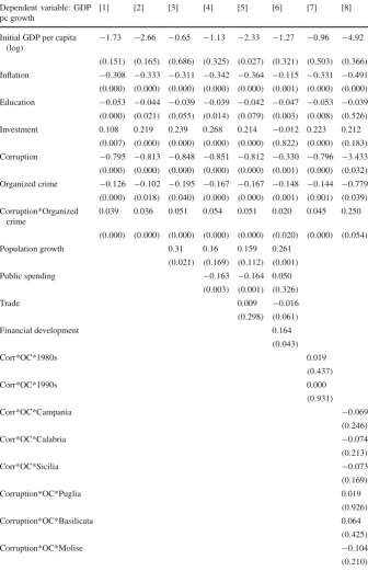
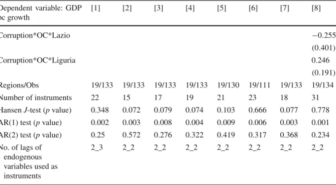
As previously discussed, a difficulty associated with the dynamic GMM estimators relates to the choice of the number of lags of the endogenous variables that are used as instruments. So far, our system-GMM results have been obtained by using a length of two to three lags in order to limit the number of instruments. As a robustness test, we reduce the length of the maximum lags to two so that we only use the second lagged value of a variable as its instrument. The results are shown in Column 2 of Table4, while Column 1 reproduces Column 5 of Panel B in Table3for comparison purposes. Our findings remain intact and the coefficient estimates are very stable.
Table 4 Robustness tests to additional controls and dummy interactions Dependent variable: GDP
pc growth
[1] [2] [3] [4] [5] [6] [7] [8] Initial GDP per capita
(log)
−1.73 −2.66 −0.65 −1.13 −2.33 −1.27 −0.96 −4.92
(0.151) (0.165) (0.686) (0.325) (0.027) (0.321) (0.503) (0.366) Inflation −0.308 −0.333 −0.311 −0.342 −0.364 −0.115 −0.331 −0.491
(0.000) (0.000) (0.000) (0.000) (0.000) (0.001) (0.000) (0.000) Education −0.053 −0.044 −0.039 −0.039 −0.042 −0.047 −0.053 −0.039
(0.000) (0.021) (0.055) (0.014) (0.079) (0.003) (0.008) (0.526) Investment 0.108 0.219 0.239 0.268 0.214 −0.012 0.223 0.212
(0.007) (0.000) (0.000) (0.000) (0.000) (0.822) (0.000) (0.183) Corruption −0.795 −0.813 −0.848 −0.851 −0.812 −0.330 −0.796 −3.433
(0.000) (0.000) (0.000) (0.000) (0.000) (0.001) (0.000) (0.032) Organized crime −0.126 −0.102 −0.195 −0.167 −0.167 −0.148 −0.144 −0.779
(0.000) (0.018) (0.040) (0.000) (0.000) (0.001) (0.001) (0.039) Corruption*Organized
crime
0.039 0.036 0.051 0.054 0.051 0.020 0.045 0.250
(0.000) (0.000) (0.000) (0.000) (0.000) (0.020) (0.000) (0.054) Population growth 0.31 0.16 0.159 0.261
(0.021) (0.169) (0.112) (0.001) Public spending −0.163 −0.164 0.050
(0.003) (0.001) (0.326)
Trade 0.009 −0.016
(0.298) (0.061)
Financial development 0.164
(0.043)
Corr*OC*1980s 0.019
(0.437)
Corr*OC*1990s 0.000
(0.931)
Corr*OC*Campania −0.069
(0.246)
Corr*OC*Calabria −0.074
(0.213)
Corr*OC*Sicilia −0.073
(0.169)
Corruption*OC*Puglia 0.019
(0.926)
Corruption*OC*Basilicata 0.064
(0.425)
Corruption*OC*Molise −0.104
Table 4 continued Dependent variable: GDP pc growth
[1] [2] [3] [4] [5] [6] [7] [8]
Corruption*OC*Lazio −0.255
(0.401)
Corruption*OC*Liguria 0.246
(0.191) Regions/Obs 19/133 19/133 19/133 19/133 19/130 19/111 19/133 19/134 Number of instruments 22 15 17 19 21 23 18 31 HansenJ-test (pvalue) 0.348 0.072 0.079 0.074 0.103 0.666 0.077 0.778 AR(1) test (pvalue) 0.002 0.003 0.008 0.004 0.009 0.006 0.003 0.001 AR(2) test (pvalue) 0.25 0.572 0.276 0.322 0.419 0.317 0.368 0.234 No. of lags of
endogenous variables used as instruments
2_3 2_2 2_2 2_2 2_2 2_2 2_2 2_2
Dependent variable is the GDP per capita growth rate.pvalues in parentheses. Constant term not reported. Regressions based on System-GMM. All control variables are instrumented for. OC measured by the baseline index, OC Index 5
In some Italian regions (for instance Puglia, Basilicata, Lazio, Liguria, Molise) organized crime is a relatively recent phenomenon. Thus, it is possible that our results may be driven by variations in organized crime across time. In order to control for this variability, we estimate the regression by adding interaction terms of corruption, organized crime and decadal dummies.27 The results are reported in Column 7 of Table4, and they show that decadal differences in organized crime do not seem to matter for growth. It is also possible that our findings are driven by regional differences in organized crime experience. We account for such regional dissimilarities by adding interaction terms of corruption, organized crime and territorial dummy variables for regions where organized criminality is more widespread.28 The results are reported in the last column of Table4, and they show that our main findings are still robust. Further, the region-specific estimates of the interaction between organized crime and corruption are not statistically significant.
6.2 Robustness to alternative measures of organized crime
For the most part of the preceding analysis, we have used OC Index 5 as our preferred measure of organized crime. It is important to verify that our results can be established
27 Since our baseline measure of organized crime is available for the period 1983–2009, we account for
the two decades 1980s and 1990s, excluding the 2000s so as to avoid the so-called dummy-trap.
28 As before, the regions have been classified on the base of the data on mafia-type criminal association
using other measures that have been adopted in the literature. To this end, we construct additional indices of organized crime by considering different combinations of Mafia-related offences and applying them in estimations of Eq. (1). Being highly corMafia-related, these indices are not expected to produce results that are substantially different from those based on our OC Index 5. Table5confirms this.
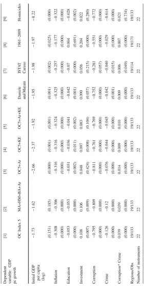
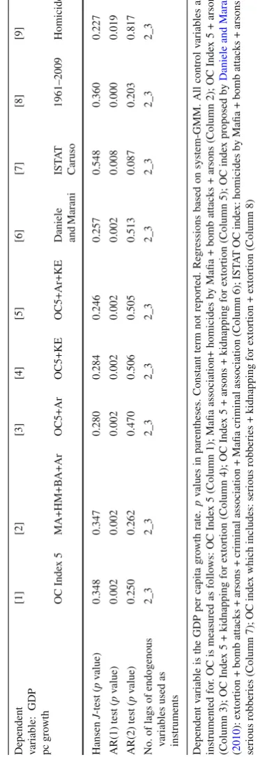
Column 1 replicates Column 5 of Table3(Panel B) for comparison. As discussed earlier, this baseline measure is constructed as the sum of official data recorded on five different types of crime that are defined as being proof, or deemed symptomatic, of the presence of criminal organizations (i.e., criminal association, Mafia criminal associa-tion, homicides by Mafia, bomb attacks, and extortion). Column 2, instead, reports the results using an index that excludes criminal association and extortion, but which prox-ies the latter by arson and bomb attacks as the primary means of exacting payments from businesses (e.g., Confesercenti 2009; Daniele and Marani 2010). The subse-quent columns take OC Index 5 and add successively arson (Column 3), kidnapping for extortion (Column 4), and both arson and kidnapping for extortion (Column 5).
Added to the above are results based on three further measures of organized crime. The first of these (Column 6) is the index of organized crime proposed byDaniele and Marani(2010). This differs from our baseline index in its exclusion of homicides by the Mafia but inclusion of arson. The second (Column 7) is the measure produced by the Italian National Institute of Statistics (ISTAT), as used byCaruso(2008). This is based on the definition of criminal organization given by the Italian Minister of Interiors, and includes the crimes of homicides by the Mafia, bomb attacks, arson and serious robberies.29The third (Column 8) is an index constructed more broadly from data on extortion, kidnapping for extortion and serious robberies (available from CRENOS). This is not strictly associated with organized crime, but may be regarded as closely proxying it for reasons given earlier, and has the appeal of covering a relatively long time span (beginning from 1961).
As Table5shows, the use of alternative measures of organized crime makes little difference to our original results. The growth effects of our three key variables— organized crime, corruption and the interaction between these—remain statistically significant and in the same direction (i.e., negative, negative and positive). An addi-tional set of results presented in Column 9 of the Table relate specifically to the interaction term. One might raise the question about whether the effect of this term is specific to organized crime, or whether it extends to other types of crime. To address this question, we conduct a falsification test, where organized crime is replaced by a measure of normal crime. A natural choice of the latter is intentional homicide, given that such crime is well-reported and given that it has a well-known distortionary effect on growth (e.g.,Cárdenas and Rozo 2008; Detotto and Otranto 2010). Our results confirm this effect, whilst also demonstrating that its magnitude is not conditional on the presence or absence of corruption. In other words, the interaction term is not statistically significant. This implies that our previously robust finding of a positive
29 Rather than using directly the index given by ISTAT, we construct an index as the sum of organized crime
Ta b le 5 Rob u stness to alternati v e measures of (or g anized) crime
Dependent variable:
[image:20.439.63.345.49.608.2]Ta
b
le
5
continued
Dependent variable:
[image:21.439.59.246.62.605.2]Table 6 Robustness to alternative PCA indexes of organized crime Dependent variable:
GDP pc growth
[1] [2] [3] [4] [5]
Index 3 Index 4 Index 5 Index 6 ISTAT Index Initial GDP pc (log) −0.28 −0.82 −0.22 −1.67 −2.48
(0.745) (0.411) (0.805) (0.080) (0.000) Inflation −0.35 −0.363 −0.349 −0.373 −0.255
(0.000) (0.000) (0.000) (0.000) (0.000) Education −0.083 −0.086 −0.083 −0.080 −0.060
(0.000) (0.000) (0.000) (0.000) (0.000) Investment 0.188 0.215 0.188 0.197 −0.001
(0.000) (0.000) (0.000) (0.000) (0.967) Corruption −0.225 −0.137 −0.197 −0.144 −0.279
(0.000) (0.002) (0.002) (0.079) (0.000) Organized crime −0.609 −0.515 −0.463 −0.571 −0.765
(0.000) (0.000) (0.000) (0.000) (0.000) Corruption*Organized crime 0.268 0.138 0.174 0.105 0.112
(0.000) (0.000) (0.000) (0.000) (0.000) Regions/Obs 19/133 19/133 19/133 19/133 19/133
Number of instruments 22 22 22 22 22
HansenJ-test (pvalue) 0.318 0.272 0.280 0.239 0.046 AR(1) test (pvalue) 0.002 0.002 0.002 0.001 0.004 AR(2) test (pvalue) 0.893 0.132 0.259 0.239 0.273 No. of lags of endogenous
variables used as instruments
2_3 2_3 2_3 2_3 2_3
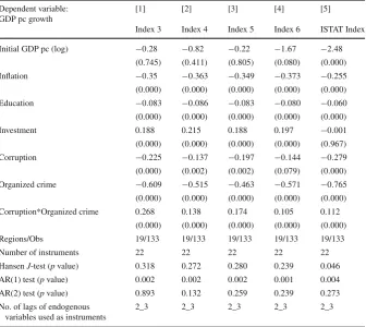
Dependent variable is the GDP per capita growth rate.pvalues in parentheses. Constant term not reported. Regressions based on system-GMM. All control variables are instrumented for. Index 3: PCA of Mafia criminal association, homicides by Mafia, criminal association; Index 4: PCA of Mafia criminal association, homicides by Mafia, criminal association, bomb attacks; Index 5: PCA of crime variables in baseline measure OC Index 5; Index 6: PCA of Mafia criminal association, homicides by Mafia, bomb attacks, arsons; ISTAT Index: PCA of crime variables in ISTAT Index
interaction term is likely to reflect an association between organized crime (rather than general crime) and corruption.
To this point, our indices for organized crime have been constructed as the sum of various Mafia-related crimes. As a final robustness check of our results, we use measures of organized crime obtained from Principal Component Analysis (PCA).30 Table6reports our results using alternative measures of organized crime based on the PCA procedure. Column 1 relates to crimes of criminal assocation, Mafia association
30 Generally speaking, PCA is a statistical technique that is used for data reduction. It is appropriate
and Mafia homicides. Column 2 extends this to include bomb attacks, whilst Column 3 makes a further extension to include extortion (corresponding to our baseline OC Index 5). Column 4 adds arson to the list of offences and excludes criminal association and extortion, and Column 6 refers to the list of offences suggested by ISTAT. In each and every case, our main results are unchanged.
7 Conclusion
This paper has sought to cast further light on the growth implications of organized crime and its interaction with corruption. The adverse effects of these two phenomena on growth and development are well-documented, and the fight against each of them remains high on the agendas of national and international agencies. What is less well-understood is the extent to which their impacts might be reinforced or subdued through linkages between them. The mechanics of this ambiguity have been documented in a companion paper, by BNR, and briefly summarized in this study. In this paper, our primary objective is to take the analysis further in an effort to resolve this ambiguity. We do this by investigating empirically whether organized crime distorts economic growth by a different degree when acting alone compared to when co-existing with corruption. The long and strong presence of both these illicit activities in Italy, make this country a natural choice to apply our examination.
Open Access This article is distributed under the terms of the Creative Commons Attribution 4.0 Interna-tional License (http://creativecommons.org/licenses/by/4.0/), which permits unrestricted use, distribution, and reproduction in any medium, provided you give appropriate credit to the original author(s) and the source, provide a link to the Creative Commons license, and indicate if changes were made.
Data appendix
[image:24.439.54.384.187.561.2]See Table7.
Table 7 Description of variables and sources
Variables Description Sources
GDP growth pc Log difference of GDP per capita in thousands of millions of lire (constant 1990 prices)
ISTAT-Annals of Statistics and CRENoS-1961/2009 Initial GDP pc (log) Log of initial GDP per capita in
thousands of millions of lire (constant 1990 prices)
ISTAT-Annals of Statistics and CRENoS-1961/2009 Investment Share of gross private investment
(% of GDP)
ISTAT-Annals of Statistics and CRENoS-1961/2009 Education Percentage of population in age
range 14–18 registered in high school
ISTAT-Annals of Statistics and CRENoS-1961/2009 Inflation GDP deflator ISTAT-Annals of Statistics and
CRENoS-1961/2009 Population growth Population growth rate ISTAT-Annals of
Statistics-1961/2009 Public spending Share of total public spending (%
of GDP)
ISTAT-Annals of Statistics-1961/2009 Trade Share of trade (% of GDP) ISTAT-Annals of
Statistics-1961/2009 Financial development Share of value added of financial
and banking sector (% of GDP)
ISTAT-Annals of Statistics and CRENoS-1975/2009 Corruption Number of crimes against Public
Administration (PA) based on Statues no. 286 through 294. Excluding crimes against PA that do not involve corruption such as Statute 279 (insulting a public officer) and Statute 295 (neglect or refusal of an official duty) reported to the police, per 100,000 inhabitants. These crimes include embezzlement and misallocation of public funds
Table 7 continued
Variables Description Sources
OC Index 5 Sum of the following crimes: Mafia criminal association, homicides by Mafia, criminal association, bomb attacks, extortion (per 100,000 inhabitants)
ISTAT-Annals of Judicial Statistics-1983/2009
Extortion Number of crimes of extortion denounced (per 100,000 inhabitants)
ISTAT-Annals of Judicial Statistics-1975/2009 Criminal Association
(art.416)
Number of crimes of criminal association (per 100,000 inhabitants) defined as:“the association of three or more people who are organized in order to commit a plurality of crimes”
ISTAT-Annals of Judicial Statistics-1975/2009
Mafia Criminal Association (art.416 bis)
Number of crimes of Mafia criminal association (per 100,000 inhabitants) defined as:“the association is of the Mafia type when its components use intimidation, awe and silence in order to commit crimes, to acquire the control or the management of business activities (i.e., concessions, permissions, public contracts or other public services), to derive profit or advantages for themselves or others, to limit the freedom of exerting the right to vote, and to find votes for themselves or others during the electoral campaign.”
ISTAT-Annals of Judicial Statistics-1983/2009
Homicides by Mafia Number of homicides by mafia (per 100,000 inhabitants)
ISTAT-Annals of Judicial Statistics-1975/2009 Bomb attacks Number of bomb attacks (per
100,000 inhabitants)
ISTAT-Annals of Judicial Statistics-1983/2009 Arsons Number of arsons (per 100,000
inhabitants)
ISTAT-Annals of Judicial Statistics-1975/2009 Robberies in Banks Number of robberies in banks
(per 100,000 inhabitants)
ISTAT-Annals of Judicial Statistics-1975/2009 Robberies in Post Offices Number of robberies in post
offices (per 100,000 inhabitants)
ISTAT-Annals of Judicial Statistics-1975/2010 Kidnapping for extortion Number of kidnapping for
extortion (per 100,000 inhabitants)
Table 7 continued
Variables Description Sources
OC Index ISTAT Sum of the following crimes: homicides by Mafia, bomb attacks, arsons, serious robberies (in banks and post offices) per 100,000 inhabitants
ISTAT-Annals of Judicial Statistics-1983/2009
OC Index CRENOS Sum of the following crimes: extortion, kidnapping for extortion, serious robberies (in banks and post offices) per 100,000 inhabitants
ISTAT-Annals of Statistics and CRENoS-1961/2009
OC Index Daniele–Marani Sum of the following crimes: extortion, bomb attacks, arsons, criminal association, Mafia criminal association (per 100,000 inhabitants)
ISTAT-Annals of Judicial Statistics-1983/2009
Homicides Number of intentional homicides (per 100,000 inhabitants)
ISTAT-Annals of Judicial Statistics-1960/2010 PCA OC Index 5 Principal Component Analysis of
the crimes included in OC Index 5
ISTAT-Annals of Judicial Statistics-1983/2009
References
Ahlin, C., Pang, J.: Are financial development and corruption control substitutes in promoting growth? J Dev Econ86(2), 414–433 (2008)
Angeles, L., Neanidis, K.C.: Aid effectiveness: the role of the local elite. J Dev Econ90, 120–134 (2009) Arellano, M., Bond, S.: Some tests of specification for panel data: Monte Carlo evidence and an application
to employment equations. Rev Econ Stud58, 277–297 (1991)
Asmundo, A., Lisciandra, M.: The cost of protection racket in Sicily. Glob Crime9(3), 221–240 (2008) Barro, R.J.: Economic growth in a cross section of countries. Q J Econ106(2), 407–443 (1991) Becker, G., Stigler, G.: Law enforcement, malfeasance, and the compensation of enforces. J Leg Stud3,
1–19 (1974)
Benhabib, J., Spiegel, M.: The role of human capital in economic development. J Monet Econ34(2), 143–174 (1994)
Blackburn, K., Neanidis, K.C., Rana, M.-P.: A theory of organized crime, corruption and economic growth. Econ Theory Bull (2017). doi:10.1007/s40505-017-0116-5
Bond, S., Hoeffler, A., Temple J.: GMM estimation of empirical growth models. CEPR Discussion Paper No. 3048 (2001)
Bowles, R., Garoupa, N.: Casual police corruption and the economics of crime. Int Rev Law Econ17, 75–87 (1997)
Buscaglia, E., Van Dijk, J.J.M.: Controlling organized crime and corruption in the public sector. Forum on Crime and Society, 3(1–2). United Nations Publications (2003)
Cárdenas, M., Rozo, S.: Does crime lower growth? evidence from Colombia. Commission on Growth and Development, World Bank Working Paper No. 30 (2008)
Caruso, R.: Public spending and organized crime in Italy. A panel-data analysis over the period 1997–2003. Università Cattolica del Sacro Cuore di Milano, Institute of Political Studies (2008)
Center for the Study of Democracy: Examining the links between organised crime and corruption. Sofia: Center for the Study of Democracy (2010)
Ciconte, E.: Ndrangheta dall’unità ad oggi, Bari, ed. Laterza (1992)
Confesercenti: The hands of criminality on enterprises. SOS Enterprise XII Report, Confesercenti, Roma (2009)
Daniele, V.: Organized crime and regional development. A review of the Italian case. Trends Org Crime
3–4, 211–234 (2009)
Daniele, V., Marani, U.: Organized crime and foreign direct investments: the Italian case. CESifo Working Paper No. 2416 (2010)
Del Monte, A., Papagni, E.: Public expenditure, corruption, and economic growth: the case of Italy. Eur J Polit Econ17(1), 1–16 (2001)
Del Monte, A., Papagni, E.: The determinants of corruption in Italy: regional panel data analysis. Eur J Polit Econ23(2), 379–396 (2007)
Detotto, C., Otranto, E.: Does crime affect economic growth? Kyklos63, 330–345 (2010) Di Liberto, A.: Education and Italian regional development. Econ Educ Rev27, 94–107 (2008)
Eurobarometer: Opinions on organized, cross-border crime and corruption. Special Eurobarometer 245/Wave 64.3-TNS Opinion & Social (2006)
Fajnzylber, P., Lederman, D., Loayza, N.: What causes violent crime? Eur Econ Rev46(7), 1323–1357 (2002)
Hansen, L.: Large sample properties of generalized methods of moments estimators. Econometrica50, 1029–1054 (1982)
Kugler, M., Verdier, T., Zenou, Y.: Organized crime, corruption, and punishment. IUI, The Research Institute of Industrial Economics, Working Paper No. 600 (2003)
La Spina, A., Lo Forte, G.: I Costi dell’ Illegalità”. Rivista Economica del Mezzogiorno, 3–4, pp. 509–570. Bologna: Il Mulino (2006)
Levine, R., Renelt, D.: A sensitivity analysis of cross-country growth regressions. Am Econ Rev82, 942–963 (1992)
MacDonald, Z.: Official crime statistics: their use and interpretation. Econ J112(477), F85–F106 (2002) Mazzitelli, A.L.: Transnational organized crime in West Africa: the additional challenge. Int Aff83(6),
1071–1090 (2007)
Pinotti P.: The economic consequences of organized crime: evidence from Southern Italy. Bank of Italy (2011)
Polinsky, M., Shavell, S.: Corruption and optimal law enforcement. J Public Econ81, 1–24 (2001) Roodman, D.: How to do xtabond2: an introduction to “Difference” and “System” GMM in Stata. Working
Paper 103. Washington, DC: Centre for Global Development (2006)
Sachs, J.D., Warner, A.M.: Sources of slow growth in African economies. J Afr Econ6, 335–376 (1997) Sergi, B.S., Qerimi, Q.: Fighting corruption and organized crime as a means of socio-economic development
in South-East Europe. South-East Eur Rev2, 81–94 (2007)
Soares, R.: Development, crime and punishment: accounting for the international difference in crime rates. J Dev Econ73(1), 155–184 (2004)
United Nations: UN general assembly 94th plenary meeting, Resolution 49/159 Naples Political Declaration and Global Action against Organized Transnational Crime (1994)
Windmeijer, F.: A finite sample correction for the variance of linear two-step GMM estimators. J Econom