Simulation of Efficient Access Point Placement Strategies in Li- Fi Network using Point Processes

(1)

International Journal of Emerging Technology and Advanced Engineering

Website: www.ijetae.com (ISSN 2250-2459, ISO 9001:2008 Certified Journal, Volume 7, Issue 9, September 2017)

256

Simulation of Efficient Access Point Placement Strategies in

Li-Fi Network using Point Processes

Subhajit Adhikari

Assistant Professor, Department of Computer Science, Dinabandhu Andrews Institute of Technology and Management, Kolkata, 700094, India

Abstract— This paper aims at the simulation and comparison of different deployment strategies of optical Access Points (APs) using spatial point processes in Li-Fi networks. Poisson point process, Matérn point process Type-I and Type-II are simulated and compared accordingly. Matérn hardcore point process Type-I and Type-II overcome the problem of Poisson point process where the random points may be arbitrarily close to each other, removing the points that are less than hardcore distance, that can be defined per system per application basis. But the number of points (APs) is few in Matérn point processes that lead to poor coverage. So we present modified deployment strategies using Matérn point process that take intensity of the process, also the hardcore distance i.e. the Euclidean distance between two points and threshold value i.e. a percentage range of discarded points and give the deployment scenario of random points (i.e. APs). Performance evaluation of proposed AP placement strategies is done by different QoS parameters e.g. discard percentage and coverage etc. The hardcore distance is dynamically changed to get better deployment scenarios in terms of more coverage with adequate number of APs. Simulation results

using MATLAB are given in support.

Keywords— Li-Fi, VLC, Access Points, deployment strategies, Poisson point process, Matérn point processes, Hard core distance, coverage etc.

I. INTRODUCTION

Light-fidelity (LiFi) [1] as a variant of VLC, is a continuation of the trend to move to higher frequencies in the electromagnetic spectrum. LiFi provides high speed wireless communication with the help of uses light emitting diodes (LEDs) and speeds of over 3 Gb/s. It has an objective to unlock a huge amount of unused electromagnetic spectrum in the visible light region. An optical attocell [2] network is a very new concept which defines an indoor small cell cellular network based Visible Light Communication. As a small base station (BS) or access point (AP), an optical attocell network [3] uses each of the luminaries providing multiple wireless users within the illuminated area.

In the past, reduction in the inter-site distance of cellular base stations is an advantage of wireless cellular communication. The spectral efficiency of the network has been increased by two orders of the magnitude in the last 25 years with small cell size. Different cell layers consist of microcells, picocells and femtocells have been introduced and are referred to as heterogeneous networks. In order to overcome the interference, this small cell concept with the extension to VLC produced by the closed reuse of radio frequency spectrum in heterogeneous networks.

The optical AP is an attocell. The coverage of each single attocell is very limited, thus the system does not suffer from co-channel interference across rooms that are confined by walls. So multiple access points can be deployed to cover a given space [4].

Here only the placement strategies of Optical APs are discussed. For a random pattern, a spatial point process is a useful for modeling points. As an example, if the locations of all the people as points in a map and they reside in different places, who called emergency service in a particular day, a random pattern of points is obtained using point process. Access points can be considered as random points. So spatial point processes can be used to model the placement of access points. To represent the different deployment strategies, we use the concept of voronoi diagram [5] .

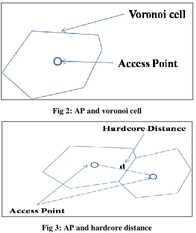
[image:1.612.348.540.575.672.2]

Each point in voronoi diagram is a Lifi access points (AP). Access points, hard core distance and voronoi diagram are represented on following figures.

(2)

[image:2.612.71.267.137.370.2]

257 Fig 2: AP and voronoi cell

Fig 3: AP and hardcore distance

In this paper, access points of LiFi network are deployed using different point processes and coverage percentage is obtained. Then new deployment strategies are proposed and simulated and coverage is also calculated.

II. LITERATURE SURVEY

In the paper [6], it is shown that in a Li-Fi network, placement of APs affects the system performance. Different scenarios are compared using different point processes for deploying Access Points. Spatial point process provides more accurate and tractable solution for network interference modeling according to them.

In paper [7], they model the placement of BS as a homogenous Poisson point process of density lamda, instead of placing BS deterministically in a grid considering the coverage. Disadvantage of Poisson point process is also discussed.

In the paper [8] , the problems of identifying neighbor and connectivity of WSNs in two dimensional space are discussed. The number of nodes (n) assumed to be distributed in region S= [0, 1] d, d=1, 2, 3, and where d=2, according to a two-dimensional homogeneous Poisson point process with density lamda(lamda=n/l2 ) . The value of lambda i.e. a certain approximation may be set by the network designer [9].

In [10] positioning techniques are used in location identification, navigation, etc. VLC has several advantages as it is low price and needs simple hardware implementation, can transmit position info through LED, it can be used in RF sensitive areas like hospital and aircrafts, due to no electromagnetic and RF interference, it has little influence of multipath interference that caused by non-line of sight, due to the main energy of indoor visible light concentrate in the line of sight link, it can provide higher precision than traditional positioning techniques that based on electromagnetic wave, also can be extended and expanded easily.

The transmitter [11] in a VLC luminaire i.e. a complete lighting unit composed of an LED lamp, ballast, housing and other components. There are two types of VLC receivers to receive the signal transmitted by an LED luminaire. Photodetector acts as photodiode or non-imaging receiver and imaging sensor acts as a camera sensor.

In the paper [12] several applications of VLC are discussed. They are underwater communication i.e. light penetrate through the water and can be used for underwater communication ,urban light infrastructure i.e. wireless communication (i.e. free of high data rate interference), cellular communication i.e. in this application street lamps(LED lamps) may be can be used both for study and internet connection (for high speed download) for a student, indoor navigation system for visually impaired, augmented reality mobile application i.e. in this application, instead of GPS, VLC can provide location information inside a building, traffic management system i.e. communication between cars and traffic lights is achieved for preventing accidents.

III. PRELIMINARY CONCEPTS

A. Poisson process

(3)

258 A Poisson point process on a set A with intensity lamda can be obtained in two steps:

 First a number N (i.e. expected number of events) is Poisson distributed with expectation λ|A|.

 Then N=n, generate X1, X2, Xn as variables that are independent and identically distributed each with a uniform distribution over A. Then set X holds points X1, X2,…, Xn as X={ X1, X2,…, Xn }.

B. Matérn point process Type-I

In this point process [14] , points from a stationary parent Poisson point process of intensity λp, are retained only if they are at distance at least δ from all other points.

C. Matérn point process Type-II

Here a random mark [14] is associated with each point, and a point of the parent Poisson process is deleted if there exist another point within the hardcore distance δ with a smaller mark.

D. Voronoi daigram

In the computational [5] geometry problem solving is done by voronoi diagram with point set and other problems about distance of geometric object.

IV. PROPOSED WORK

In this paper, different point processes are used to model the deployment of access points (APs) in optical network with voronoi diagram representation. A unit square area of 20m×20m is considered for deployment. Intensity parameter (lamda) is very much important for entire process to succeed. Firstly Poisson Point Process is used for placement of APs. Different numbers of points are obtained with different intensity values.

But a problem arrives when two random points (APs) are arbitrarily close to each other in poisson point process, coverage areas of two APs are overlapping. If overlapping can be reduced, more area can be covered with less no. of APs and that can be done using efficient AP placement strategy. In Matérn hard-core point, this limitation of poisson process is eliminated by removing the points that are at a distance less than a predefined parameter. The distance parameter is called as hard-core distance. The intensity parameter (lamda) and hard-core distance are defined per system per application basis. Simulation of three point processes is done and they are homogeneous Poisson Point Process, Matérn point process type I and type II. The result is presented in a table given below.

TABLE I

COMPARISON OF HCPP1 AS MATÉRN HARD-CORE POINT PROCESS TYPE-I AND HCPP2 AS MATÉRN HARD-CORE POINT PROCESS TYPE-II

Hard Core

distance Lamda

HCPP1 HCPP2

Analysis No

of AP s

AP density

No of AP s

AP density

1

10 11 0.0275 13 0.0325 HCPP2

50 47 0.1175 42 0.105

HCPP1

100 68 0.17 85 0.2125

HCPP2

2

10 8 0.02 10 0.025 HCPP2

50 23 0.0575 33 0.0825 HCPP2

100 32 0.08 38 0.095

HCPP2

3

10 10 0.025 9 0.0225

HCPP1

50 16 0.04 28 0.07

HCPP2

100 16 0.04 38 0.095

HCPP2

According to the paper [1] , a comparative study has been made of Matérn hard-core point process type-I and Matérn hard-core point process type-II considering Poisson point process as basis of deployment and the result is provided in the above table where hardcore distances are 1, 2 and 3 and for three different lamda values 10, 50, 100. Density of access points (APs) in Matérn hard-core point processes is compared.

APdensity=No.OfPoints/area………….. (1)

(4)

259 It is obvious that less number of access points (APs) with cell radius of 1-4 meter, are unable to provide to better coverage in a simulation area of 20m*20m. Next the coverage percentage (cp) is measured.

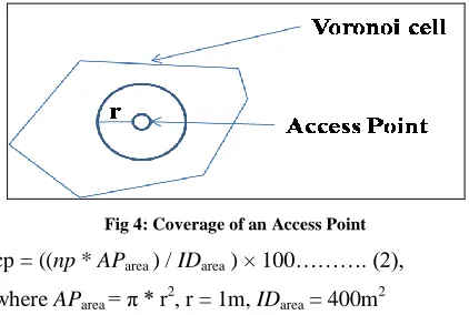
Fig 4: Coverage of an Access Point

cp = ((np * AParea ) / IDarea ) × 100………. (2), where AParea = π * r2, r = 1m, IDarea = 400m2

The coverage area of an access point is taken as disk coverage with fixed radius r. In equation (2), AParea refers to the coverage area of access points, np refers to number of access points, IDarea and means interior deployment area.

[image:4.612.62.273.190.332.2]

So firstly we deploy the access points using existing Matérn hard-core point process type-I and the coverage percentage is 25.12% and Matérn hard-core point process type-II gives the coverage percentage 29.83% where lamda is set to 100 and hardcore distance is set to 2. Then for lamda is set to 100 and hardcore distance is set to 3, coverage percentage is 12.56% in Matérn hard-core point process type-I and 27.47% in Matérn hard-core point process type-II. All the parameters are taken experimentally. The coverage percentages are obviously poor in these cases.

TABLE II

COVERAGE FOR HCPP1 AND HCPP2

Parameters HCPP1 HCPP2

Coverage (%) Coverage

(%)

Lamda=100,hardcore distance=2

25.12 29.83

Lamda=100,hardcore distance=3

12.56 27.47

To increase the coverage percentage, we propose the new method of deploying access points using Matérn hard-core point process type-I and type-II, where discard percentage (i.e. the percentage of discarded points) are calculated and compared with a threshold value which may be user defined or system or application specific.

The threshold value signifies that the discard percentage must be closest to the value so that the intended area can be fully covered with maintaining a certain level of intensity. The range is statically taken as (threshold-0.10)≤ discard percentage ≤ (threshold +0.10).This is taken for experimental and illustration purposes only. Then the hard-core distance is recomputed with new hard-hard-core which distance must be greater than 1. Next the APs are redeployed by the new hard-core distance. It has been noticed that the percentage of discarded points are also varied. This is because the percentage is calculated after deployment of APs .The objective is not to discard huge number of points, a value of discard percentage must be specified. This leads to retain more number of points in comparison with original method of Matérn point process.

V. ALGORITHM

Algorithm 1: ppp (lamda)

/* ppp defines the Poisson Point Process*/

Input: Give intensity of the point process and pass it to a function called ppp(lamda)

Output: Placement of points (APs)

Step 1: Take parameter “lamda” as intensity of the point process.

Step 2: Generate the expected number of events “N” i.e. Poisson distributed with “lamda”.

Step 3: Form an independent random sample with the N events i.e. uniformly distributed.

Step 4: Eliminate zeroes from the set of points obtained.

Step 5: Compute and plot voronoi diagram.

Algorithm 2: Mhcpp1(lamda,c,thrsh)

/*Mhcpp1 defines the Matérn hard-core point process type-I*/

Input: Give intensity of the point process, hardcore distance and threshold value and pass it to a function as Mhcpp1(lamda,c,thrsh)

Output: Voronoi diagram representation of placement of APs. Percentage of discarded points and modified hardcore distance.

Step 1 : Take parameter intensity of the point process as “lamda” and parameter “c” i.e. the hard core distance.

Step 2 : Generate the expected number of events as “N” Poisson distributed with “lamda”

Step 3 : Form an independent random sample with the N uniformly distributed events .

(5)

260 Step 5 : Loop till N

Step 6 : If dist(i,j) < c then

Step 7 : Discard jth point

Step 8 : Else

Step 9 : Retain ith point

Step 10 : End

Step 11 : Eliminate zeroes from the set of points obtained

Step 12 : Compute and plot voronoi diagram

Step 13 : Compute the percentage of the discarded points and save it to “disper”

Step 14 : If (thrsh-0.10)<=dispts and dispts<=(thrsh+0.10) then

Step 15 : Print “The hardcore distance”

Step 16 : Else

Step 17 : Set c=c-disper

Step 18 : If c>1 and dispts>(thrsh-0.10) then

Step 19 : Mhcpp1(lamda,c,thrsh)

Step 20 : End

Step 21 : End

Algorithm 3: Mhcpp2(lamda,c,thrsh)

/*Mhcpp2 defines the Matérn hard-core point process type-II*/

Input: Give intensity of the point process,hardcore distance and threshold value and pass it to a function as Mhcpp2(lamda,c,thrsh)

Output: Voronoi diagram representation consists of APs. Percentage of discarded points and modified hardcore distance.

Step 1 : Take parameter “lamda” as intensity of the point process and parameter “c” as hard core distance.

Step 2 : Generate the number of points as variable “N” i.e. Poisson distributed with “lamda”.

Step 3: Form an independent random sample with the N events i.e. uniformly distributed.

Step 4 : Compute the number of points in npts and save it as “up”.

Step 5 : Generate random numbers i.e. random mark of each points with range from 1 to up and save it to a variable “u”.

Step 6 : Compute Euclidean distance between two points i and j as “dist”.

Step 7 : Loop till N

Step 8 : If dist(i,j) < c and u(j)<u(i) then

Step 9 : Discard jth point

Step 10 : Else

Step 11 : Retain ith point

Step 12 : End

Step 13 : Eliminate zeroes from the set of points obtained

Step 14 : Compute and plot voronoi diagram

Step 15 : Compute the percentage of the discarded points and save it to “disper”

Step 16 : If (thrsh-0.10)<=dispts && dispts<=(thrsh+0.10) then

Step 17 : Print “Hardcore distance”

Step 18 : Else

Step 19 : Set c=c-disper

Step 20 : If c>1 and dispts>(thrsh-0.10) then

Step 21 : Mhcpp2(lamda,c,thrsh)

Step 22 : End

Step 23 : End

VI. SIMULATION RESULT

The placement strategies of APs are simulated in MATLAB R2015b. Defined functions are used for simulation. The function “poissrnd (lamda)” is used for generating number of Poisson points with lamda which represents the intensity of the point process. The random function (i.e. “rand()”) is used then to produce the coordinates of the previously generated points. The Matérn type I hard-core point process and Matérn type II hard-core point process are implemented by the functions “Mhcpp1” and “Mhcpp2” respectively. For example the simulation result of Mhcpp1(100,3,0.50) is given below. The parameters are given by user.

(a)Poission Point process

(6)

261 Fig 5: In the voronoi diagram,the dots are representing the optical APs in modified Matérn type I hard-core point process (size of deployment area 20m x 20m)

In the above figure 5, in the first trail the hardcore distance is set to 3. Then the placement of APs are done. Then the percentage of discarded points (i.e. APs) is obtained. The condition is that if the percentage lies between the range specified, the placement scenario is accepted and if not, then the function calls itself for the second trail until the condition is satisfied. Here the threshold value is taken as 0.50 for experimental purpose. So the discard percentage must lie between 0.40 and 0.60.The placement process is succeeded after some trails because the no of access points (APs) are adequate for deployment. In each trail the hardcore distance is changed subtracting the discard percentage. Lastly the hardcore distance is modified and set to 1.3900 and discard percentage is obtained as 0.5200. This value is between 0.40<0.52<0.60. So the discard percentage is accepted.

(a)Poission Point process

[image:6.612.62.276.363.610.2]

(b)Modified method using Matérn type II hard-core point process

Fig 6: In the voronoi diagram, the dots are representing the optical APs in modified Matérn type II hard-core point process (size of deployment area 20m x 20m)

In the above figure 6, According to Mhcpp2(100,3,0.50), the function for Matérn type II hard-core point process gives the result. Hardcore distance is modified to 2.4900. Discard percentage is 0.4900.

This value is between 0.40<0.4900<0.60. So the discard percentage and the placement scenario is accepted.

VII. OUR CONTRIBUTION

With adequate number of access points in our proposed method, the coverage area is increased. The coverage percentage is obtained in our simulation, given in the following table.

TABLE III

COVERAGE FOR MODIFICATION OF HARDCORE POINT PROCESS WITH MHCPP1 AND MHCPP2

Parameters MHCPP1 MHCPP2

Coverage (%)

Lamda=100,hard core distance=1.31

49.455 51.87

Lamda=100,hard core distance=1.34

40.82 32.97

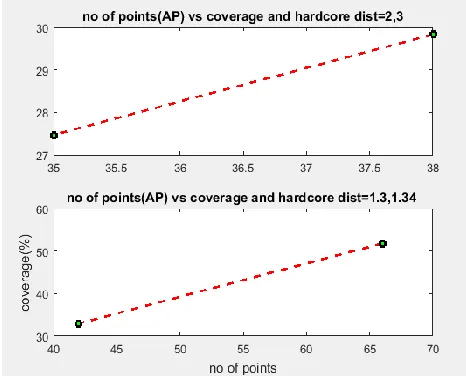
We have also compared the existing algorithms of point process and our new method of deployment according to coverage and two graphical representations are provided below.

Fig 7: Comparison of coverage percentage of existing hardcore point process-I with hardcore distance=2,3 and our proposed method with

hardcore distance=1.3,1.34

[image:6.612.327.560.415.582.2]

(7)

[image:7.612.51.284.249.437.2]

262 The two coverage percentages are depicted using a graph given below i.e. In second case, we simulate the deployment using the hardcore point process-II with lamda is set to 100, hardcore distance is set to 2,3. Then the coverage is recorded. Next we simulate our proposed method of deployment with lamda is set to 100, hardcore distance is modified to 1.3,1.34 and discard percentage 0.50 and we get the coverage.. The two coverage percentages are depicted using a graph given below i.e.

Fig 8: Comparison of coverage percentage of existing hardcore point process-II with hardcore distance=2,3 and our proposed method with

hardcore distance=1.3,1.34

From the above two graphs, it has been observed that our proposed method gives better coverage with dynamically changed hardcore distance.

VIII. CONCLUSION

Placement of Access Points is very important for area coverage in a Li-Fi network considering deployment of adequate number of APs. Our proposed method of deployment strategies using Matérn processes give the desired number of APs solving the problem of traditional Matérn point process which gives less number of points (i.e. APs) with fixed value of hardcore distance decided at the beginning of the process. In this paper we use the concept of changing hardcore distance dynamically to obtain a range of percentage of discarded points (i.e. Access Points) during deployment process. Experimental results prove the efficiency of proposed Access Point placement strategies having better coverage. The deployment of APs is also more accurate.

Improvements can be done to the process of modification of hardcore distance in point processes according to have better coverage.

REFERENCES

[1] Haas, H., 2013. High-speed wireless networking using visible light.

SPIE Newsroom, 19, doi: 10.1117/2.1201304.004773.

[2] Chen, C., Basnayaka, D.A. and Haas, H., 2016. Downlink

performance of optical attocell networks. Journal of Lightwave Technology, 34(1), pp.137-156,doi: 10.1109/JLT.2015.2511015.

[3] Chen, C., Videv, S., Tsonev, D. and Haas, H., 2015. Fractional

frequency reuse in DCO-OFDM-based optical attocell networks. Journal of Lightwave Technology, 33(19), pp.3986-4000,doi: 10.1109/JLT.2015.2458325.

[4] Tsonev, D., Videv, S. and Haas, H., 2013, December. Light fidelity

(Li-Fi): towards all-optical networking. In SPIE OPTO (pp.

900702-900702). International Society for Optics and Photonics,

doi:10.1117/12.2044649.

[5] Chang, Jun, et al. "Simulation of worst and best-case coverage for wireless sensor network." Information Networking and Automation (ICINA), 2010 International Conference on. Vol. 2. IEEE, 2010,doi: 10.1109/ICINA.2010.5636508.

[6] Haas, H., Yin, L., Wang, Y. and Chen, C., 2016. What is LiFi?.

Journal of Lightwave Technology, 34(6), pp.1533-1544,doi: 10.1109/JLT.2015.2510021.

[7] Andrews, J.G., Baccelli, F. and Ganti, R.K., 2011. A tractable

approach to coverage and rate in cellular networks. IEEE Transactions on Communications, 59(11), pp.3122-3134,doi: 10.1109/TCOMM.2011.100411.100541.

[8] Qu, Y., Fang, J. and Zhang, S., 2012. Identifying neighbor and

connectivity of wireless sensor networks with poisson point process.

Wireless Personal Communications, 64(4), pp.795-809,doi:

10.1007/s11277-010-0220-4.

[9] Santi, P. and Blough, D.M., 2003. The critical transmitting range for

connectivity in sparse wireless ad hoc networks. IEEE transactions

on Mobile Computing, 2(1), pp.25-39,doi:

10.1109/TMC.2003.1195149.

[10] Chunyue, W., Lang, W., Xuefen, C., Shuangxing, L., Wenxiao, S.

and Jing, D., 2015. The research of indoor positioning based on visible light communication. China Communications, 12(8), pp.85-92,doi: 10.1109/CC.2015.7224709.

[11] Pathak, P.H., Feng, X., Hu, P. and Mohapatra, P., 2015. Visible light

communication, networking, and sensing: A survey, potential and challenges. ieee communications surveys & tutorials, 17(4), pp.2047-2077,doi: 10.1109/COMST.2015.2476474.

[12] Singh, S., Kakamanshadi, G. and Gupta, S., 2015, December.

Visible Light Communication-an emerging wireless communication technology. In Recent Advances in Engineering & Computational Sciences (RAECS), 2015 2nd International Conference on (pp. 1-3). IEEE,doi: 10.1109/RAECS.2015.7453409.

[13] Keeler, H. P. (2016). Notes on the Poisson point process. Technical

Reports, Weierstrass Institute.

[14] Haenggi, M., 2011. Mean interference in hard-core wireless