Gong, C. and Tao, D. and Maybank, Stephen and Liu, W. and Kang, G. and
Yang, J. (2016) Multi-modal curriculum learning for semi-supervised image
classification. IEEE Transactions on Image Processing 25 (7), pp.
3249-3260. ISSN 1057-7149.
Downloaded from:
Usage Guidelines:
Please refer to usage guidelines at
or alternatively
Multi-modal Curriculum Learning for
Semi-supervised Image Classification
Chen Gong, Dacheng Tao,
Fellow, IEEE,
Stephen J. Maybank,
Fellow, IEEE,
Wei Liu,
Member, IEEE,
Guoliang Kang, and Jie Yang
Abstract—Semi-supervised image classification aims to classify a large quantity of unlabeled images by harnessing typically scarce labeled images. Existing semi-supervised methods often suffer from inadequate classification accuracy when encountering difficult yet critical images such as outliers, because they treat all unlabeled images equally and conduct classifications in an imperfectly ordered sequence. In this paper, we employ the curriculum learning methodology by investigating the difficulty of classifying every unlabeled image. The reliability and discrim-inability of these unlabeled images are particularly investigated for evaluating their difficulty. As a result, an optimized image sequence is generated during the iterative propagations, and the unlabeled images are logically classified from simple to difficult. Furthermore, since images are usually characterized by multiple visual feature descriptors, we associate each kind of features with a “teacher”, and design a Multi-Modal Curriculum Learning (MMCL) strategy to integrate the information from different feature modalities. In each propagation, each teacher analyzes the difficulties of the currently unlabeled images from its own modality viewpoint. A consensus is subsequently reached among all the teachers, determining the currently simplest images (i.e. a curriculum) which are to be reliably classified by the multi-modal “learner”. This well-organized propagation process leveraging multiple teachers and one learner enables our MMCL to outperform five state-of-the-art methods on eight popular image datasets.
Index Terms—Curriculum learning, Semi-supervised learning, Multi-modal, Image classification.
I. INTRODUCTION
C
LASSIFYING natural images into meaningful categories has always been a dominant topic in computer vision research. With the emergence of large image collections andThis research is supported by NSFC of China (No: 61572315), 973 Plan of China (No. 2015CB856004), and Australian Research Council Projects DP-140102164, FT-130101457, and LE-140100061.
C. Gong is with the Institute of Image Processing and Pattern Recognition in Shanghai Jiao Tong University. He is also with the Centre for Quantum Computation & Intelligent Systems and the Faculty of Engineering and Information Technology, University of Technology Sydney, 81 Broadway Street, Ultimo, NSW 2007, Australia. (e-mail: [email protected]).
D. Tao and G. Kang are with the Centre for Quantum Computation & Intel-ligent Systems and the Faculty of Engineering and Information Technology, University of Technology Sydney, 81 Broadway Street, Ultimo, NSW 2007, Australia (e-mail: [email protected]; [email protected]).
S. Maybank is with the School of Computer Science and Information Systems, Birkbeck, University of London, Malet Street, London WC1E 7HX, UK. (email: [email protected]).
W. Liu is with the IBM T. J. Watson Research Center, 1101 Route 134 Kitchawan Rd, Yorktown Heights, NY 10598, USA (e-mail: [email protected]).
J. Yang is with the Institute of Image Processing and Pattern Recognition, Shanghai Jiao Tong University, China, 200240 (e-mail: [email protected]). Corresponding authors: Jie Yang ([email protected]) and Dacheng Tao ([email protected]).
vigorous development of the Internet, the available labeled images are usually inadequate for training a supervised clas-sifier that has to deal with a dramatic growth in new images. Furthermore, labeling more images will incur high time and monetary costs. To address this problem, semi-supervised image classification has been developed to explicitly exploit the information revealed by both limited labeled images and sufficient unlabeled images [1], [2], [3], [4], [5], [6], [7].
Given labeled image set L of size l and unlabeled image set U of size u, conventional semi-supervised image classi-fication is usually conducted on a weighted similarity graph
G=hV,Ei[1], [8], [9], whereV is the node set representing the n = l +u images, and E is the edge set encoding the pairwise similarities between these images. The target is to iteratively propagate the labels from L to U so that all the elements in U can be precisely classified. However, existing methods [1], [8], [9] often yield unsatisfactory results, as they are very likely to make incorrect classifications on “outliers” or “bridge examples” (e.g.images that share similar properties with multiple classes). This is because existing methods treat all the unlabeled images equally without considering the difficulty or reliability of their classification. As a result, the images are classified in imperfect order, which leads to the error-prone classification of difficult but critical images such as the aforementioned “outliers” and “bridge examples”. Such errors have an adverse impact on the accurate prediction of the labels of the remaining unlabeled images.
Labeled
Unlabeled
Labeled
Unlabeled
Modality 1 (PHOG)
…
(1)
S
( )v
S
( )V
S
Curriculum
(simple unlabeled images)
…
(1)
( )V
(1)
F
Agreed curriculum
( )V
F
( )v
F
F
Learning feedback
*Conf(
F
)
S
Multi-modal curriculum generation
Multi-modal learning
( )v
Modality vModality V
(LBP)
*
S
(1)G
( )V
[image:3.612.102.510.56.277.2]G
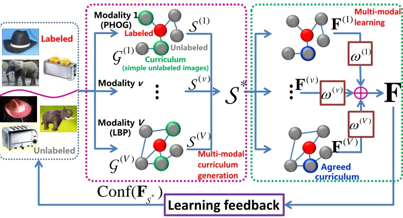
Fig. 1. The framework of our algorithm. All the labeled and unlabeled images are described byV different modalities (i.e.features). The labeled images and unlabeled images are represented by red and grey balls, respectively. Among the unlabeled images, the curriculum of each modality and the agreed curriculum S∗are further surrounded by green and blue rings accordingly. The multi-modal curriculum generation step and multi-modal learning step are marked with
magenta and green dashed boxes.
In detail, we build V graphsG1,· · · ,GV corresponding to
V modalities over the images inL ∪ U (see Fig. 1). The state-of-the-art label propagation approach [11] is applied to these V modalities to form a multi-modal semi-supervised learner, which can iteratively classify the unlabeled images. Besides, multiple “teachers” are incorporated to allocate the simplest unlabeled images to this stepwise semi-supervised learner. Here the simplest unlabeled images constitute a curriculum as they should be “learned” by the learner as required by the teachers. In each propagation, the difficulties of unlabeled images (grey balls) are evaluated by allV teachers according to their reliability and discriminability w.r.t. the labeled images (red balls), and the curriculum images decided by every individual teacher are denoted by the setS(v)(v= 1,· · ·, V)
(gray balls with green rings). An optimal curriculumS∗ (gray
balls with blue rings) agreed by all the teachers is then established based on every individual teacher’s decision. After that, the learner classifies the images in S∗ by respectively
propagating the labels fromLtoS∗inV different modalities,
and the obtained results are recorded in the label matrix
F(v)∈Rn×c (v= 1,· · ·, V, andc is the number of classes). This is also known as multi-modal learning. The integrated label matrix F∈Rn×c is the sum ofF(1),· · · ,F(V)weighted byω(1),· · · , ω(V), respectively. Finally, the learning feedback is delivered to teachers to assist them to correctly determine the subsequent simplest curriculum. This process iterates until all the images in U have been selected, and the label matrix thus produced is denoted byF¯. The(i, j)-th element inF¯ (or
F(v) and Fmentioned above) encodes the probability of the
i-th imagexi belonging to the j-th classCj.
Due to the wisdom of multiple teachers, the difficulties of unlabeled images are comprehensively evaluated, and these images are logically propagated from simple to difficult with
the updated curriculums. Our algorithm consequently achieves higher classification accuracy than other typical methods, as revealed by empirical validation. The advantage of multi-modal curriculum over single-multi-modal curriculum is also demon-strated in the experiments.
II. RELATEDWORK
In this section, we review some representative existing lit-eratures of semi-supervised image classification, multi-modal learning and curriculum learning, as they are related to this work.
A. Semi-supervised Image Classification
Semi-supervised learning (SSL) [12] has been studied for a long history, which aims to classify a massive number of unlabeled examples given the existence of only a few labeled examples. Although the massive unlabeled examples do not have explicit labels, they convey the distribution information of the entire dataset, which can be exploited for accurate clas-sification. Existing SSL algorithms can be roughly attributed to three categories: self-training [13], low density separation [14], [15], [16], and graph-based methods [17], [18], [19].
which make one class different from another. Fergus et al. [3] developed a scalable graph-based algorithm that has linear complexity with regard to the number of images. The spectral property of the graph is properly utilized to handle the large-scale image data. Other representative works include [5], [21], [22], [23].
B. Multi-modal Learning
In practical applications, data is often obtained from mul-tiple sources rather than a single source. One common way to process such multi-modal data is to concatenate the feature vectors associated with different sources into a long vector. However, this concatenation is highly intuitive and ignores the particular statistical property of an individual view, there-fore it can hardly obtain satisfactory performance. Multi-modal learning (MML) is therefore proposed to explicitly fuse the complementary information from different modalities to achieve improved performance. MML is essentially multi-view learning, and the relevant algorithms can be classified into three groups [24]: co-training [25], [26], multiple kernel learning [27], and subspace learning [28]. Co-training ap-proaches train alternately to maximize the mutual agreement on different modalities of the unlabeled data. Multiple kernel learning straightforwardly corresponds to multiple modalities and elegantly combines kernels of different modalities to achieve improved performance. Subspace learning assumes that there is a latent subspace shared by multiple modali-ties and the input modalimodali-ties are generated from this low-dimensional latent subspace.
MML has been widely adopted in semi-supervised image classification such as modal SSL [4], adaptive multi-modal SSL [1], and multi-view vector-valued manifold reg-ularization [29]. Of these, [4] is based on a multiple kernel classifier fusing both image content and its descriptive key-words. The work of [1] integrates various heterogeneous visual features via graph fusion, and then deploys label propagation [18] to infer the class labels of unlabeled images. By utiliz-ing the vector-valued functions, [29] proposes a multi-modal algorithm for multi-label image classification.
C. Curriculum Learning
Curriculum learning aims to improve the learning per-formance by designing suitable curriculums from simple to difficult for the stepwise learner. This learning approach was proposed by [10], which hypothesizes that curriculum learning is able to boost the convergence speed of the training process as well as find a better local minima than the existing solvers for non-convex problems. The self-paced learning proposed by Kumar et al. [30] can be regarded as an implementation of curriculum learning, which was extended by [31], [32] afterwards. Besides, the teaching-to-learn and learning-to-teach framework developed by Gong et al. [33], [34] also follows the idea of curriculum learning, and this paper is the extension of [33] to the multi-modal situation.
Up to now, curriculum learning has been applied to visual category discovery [35], object tracking [36], and multimedia
retrieval [37]. However, none of the existing curriculum learn-ing algorithms can handle multi-modal data, or touch semi-supervised image classification.
III. OURAPPROACH
For each feature modality (indexed by v = 1,· · ·, V), we construct a similarity graph G(v) by the recently proposed
adaptive edge weighting [38], and the associated adjacency matrix isW(v) with the(i, j)-th element W(v)
ij representing
the similarity between imagesxiandxj in terms of modality
v. The graph Laplacian is L(v)=D(v)−W(v) where D(v)
is the degree matrix with diagonal elements computed by
D(iiv)=Pn
j=1W (v)
ij .
A. Single-modal Curriculum Generation
We start by elaborating the curriculum generation on single feature modality, so the superscript(v)in previous notations is temporarily dropped in this section. The purpose of curriculum generation is to pick up the simplest curriculumS ⊂ U in each propagation. To this end, the reliability and discriminability
of every unlabeled image are investigated by the “teacher” to make a selection.
Specifically, we assign a random variableyi to each image
xi, and view the propagations on G as a Gaussian
pro-cess [39]. Therefore, this Gaussian propro-cess is modeled as a multivariate Gaussian distribution over the random variables
y= (y1,· · ·, yn)>, which has a concise form y∼ N(0,Σ)
with its covariance matrix being Σ= (L+I/κ2)−1 (Iis the
identity matrix). The parameterκ2controls the “sharpness” of
the distribution and is fixed at 100 throughout this paper. A curriculum S is reliable w.r.t. the labeled set L if the conditional entropy H(yS|yL) is small, where yS and
yL denote the subvectors of y corresponding to S and L,
respectively. This is because small H(yS|yL) suggests that
the curriculum set S comes as no “surprise” to the labeled setL. Besides, a curriculum is discriminable if the included images are significantly inclined to certain classes.
Reliability. By using the property of multivariate Gaussian [40], the most reliable curriculum can be found by optimizing:
min
S⊂U H(yS|yL)
⇔min
S⊂U H(yS∪L)−H(yL)
⇔min S⊂U
s+l
2 1 + ln 2π
+1 2ln
ΣS∪L,S∪L
−
l
2 1 + ln 2π
+1 2ln
ΣL,L
⇔min S⊂U
s
2 1 + ln 2π
+1 2ln
ΣS∪L,S∪L
ΣL,L
,
(1)
whereΣL,L andΣS∪L,S∪L are submatrices ofΣ associated
with the corresponding subscripts. By further partitioning
ΣS∪L,S∪L =
Σ S,S ΣS,L ΣL,S ΣL,L
where ΣS,S is the submatrix of
Σ corresponding toS, we have
|ΣS∪L,S∪L|
|ΣL,L| =
|ΣL,L|
ΣS,S−ΣS,LΣ
−1
L,LΣL,S
|ΣL,L|
=ΣS|L
where ΣS|L is the covariance matrix of the conditional distribution p(yS|yL) and is naturally positive semidefinite.
Therefore, the problem (1) is equivalent to
min
S⊆U tr ΣS,S −ΣS,LΣ −1
L,LΣL,S. (2)
Discriminability. The tendency of an image xi belonging to
a class Cj is modeled by the average commute time between
xiand all the images in Cj, which is formally represented by
¯
T(xi,Cj) =
1
nCj X
xi0∈Cj
T(xi,xi0). (3)
In Eq. (3),nCj denotes the number of images in the classCj;
T(xi,xi0)is the commute time [41] between images xi and
xi0, which is defined by
T(xi,xi0) =
n
X
k=1
h(λk) uki−uki0
2
,
where 0 = λ1 ≤ · · · ≤ λn are the eigenvalues of L, and
u1,· · ·,un are the associated eigenvectors; uki denotes the i
-th element of uk; h(λk) = 1/λk if λk 6= 0 and h(λk) = 0
otherwise.
Therefore, supposeC1andC2 are the two closest classes to
xi ∈ U measured by average commute time, then xi is
dis-criminable if the gapM(xi) = ¯T(xi,C2)−T¯(xi,C1)is large.
That is, the simplest curriculum in view of discriminability is found by solving
min S={xik∈ U }s
k=1
s
X
k=1
1/M(xik), (4)
wheresis the amount of images in the set S.
By combining Eqs. (2) and (4), we arrive at the following optimization problem:
min S={xik∈ U }s
k=1
tr ΣS,S−ΣS,LΣL−,1LΣL,S+
s
X
k=1
1/M(xik).
(5)
In each propagation, the seed labels will be propagated to the unlabeled images that are direct neighbors (denoted by the neighbouring set B) of L on graph G, so we only need to choose sdistinct images from B. Therefore, we introduce a binary selection matrix S∈ {1,0}b×s (b is the size of the
set B) such that S>S=Is×s. The element Sij = 1 means
that the i-th image in B is selected as the j-th element in the curriculum S. The orthogonality constraint S>S=Is×s
imposed onSensures that every image is selected only once in S. The problem (5) is subsequently reformulated to the following matrix form:
min
S tr S
>Σ
B,BS−S>ΣB,LΣ−L,1LΣL,BS + tr S>MS
,
s.t. S∈ {1,0}b×s, S>S=Is×s,
(6)
where M ∈ Rb×b is a diagonal matrix with the diagonal elements Mii = 1/M(xi) for any xi ∈ B. By denoting
R=ΣB,B−ΣB,LΣL−,1LΣL,B+M, the curriculum selection
model for single-modal case is simplified as
min
S tr S
>RS
,
s.t. S∈ {1,0}b×s, S>S=Is×s. (7)
B. Multi-modal Curriculum Generation
Single-modal curriculums cannot always render satisfactory performance (demonstrated in Section IV-A), we therefore extend the single-modal model (7) to multi-modal cases. The high level idea is to force theV teachers to reach a consensus on selecting the optimal curriculumS∗. This is formulated as
an optimization problem, which can be solved by relaxing the binary selection matrices to continues ones, and then conduct-ing the standard alternatconduct-ing minimization. Each subproblem in the alternating minimization is constrained by an orthogonal constraint, and can be optimized by the existing solver on matrix manifold.
In order to regulate the selection matrices S(v) (v = 1,· · ·, V) generated byV teachers to compromise to a common
S∗, we define the following optimization:
min
S(1),···,S(V),S∗
V
X
v=1
tr S(v)>R(v)S(v)
+β
V
X
v=1
S
(v)−S∗
2 F s.t. S∗∈ {1,0}b×s, S∗>S∗=I
s×s,
S(v)∈ {1,0}b×s, S(v)>S(v)=I
s×s, forv= 1,· · ·, V.
,
(8)
where the first term in the objective function shares the similar purpose with the objective in Eq. (7), which requires all teachers to select the simplest images according to their modality viewpoints. The second term makes the teachers maximally agree with each other and produce the consistent curriculum, where “k·kF” computes the Frobenius norm.β >0
is the trade-off parameter. However, The binary constraints turn the optimization (8) into an integer programming which is generally NP-hard. To make problem (8) tractable, we relax the discrete constraints to continuous nonnegative constraints and achieve the following expression:
min
S(1),···,S(V),S∗
V
X
v=1
tr S(v)>R(v)S(v)
+β
V
X
v=1
S
(v)
−S∗
2 F s.t. S∗≥Ob×s, S∗>S∗=Is×s,
S(v)≥Ob×s, S(v)>S(v)=Is×s, forv= 1,· · ·, V
,
(9)
where O denotes the zero matrix. A local minimizer of problem (9) can be obtained by alternatively optimizing
S(1),· · ·,S(V), andS∗ with other variables remaining fixed. Updating S(v). To obtain the optimal selection matrix S(v)
where v takes a value from 1,· · ·, V, we treat S∗ and S(v0)
(v06=v) as constant variables, and then the S(v)-subproblem
is derived as
min
S(v) tr S
(v)>R(v)S(v)
+β S
(v)−S∗
2 F s.t. S(v)≥Ob×s, S(v)>S(v)=Is×s.
The nonnegative constraint in the above optimization can be easily tackled by the method of augmented Lagrangian multiplier (ALM). The main idea of ALM is to transform a constrained optimization problem into a non-constrained problem by incorporating penalty terms. Compared with the traditional Lagrangian method, ALM adds an additional quadratic penalty function to the objective, which leads to faster convergence rate and lower computational cost [42]. However, in our case the orthogonal constraint cannot be directly degenerated into the augmented Lagrangian function because it defines a nonconvex feasible region on the Stiefel manifold (the Stiefel manifold is the set of all m1×m2
ma-trices satisfying the orthogonal constraint, i.e.St(m1, m2) =
X∈Rm1×m2:X>X=I
m2×m2 ). As a result, we only in-corporate the nonnegative constraint into the augmented La-grangian function and project the result produced by gradient descent back onto the Stiefel manifold in each iteration. The augmented Lagrangian function is
L(S(v),Λ(v),T(v), σ(v))
= tr S(v)>R(v)S(v)+β
S
(v)−S∗
2 F + tr Λ(v)>(S(v)−T(v))
+σ (v) 2
S(v)−T(v)
2 F,
whereΛ(v)∈Rb×sis the Lagrangian multiplier,T(v)∈Rb×s is a nonnegative auxiliary matrix, and σ(v)>0 is the penalty
coefficient. Therefore, S(v)is updated by
S(v):= ProjSthS(v)−τ∇S(v)L
S(v),Λ(v),T(v), σ(v)i,
(11) where ∇S(v)L S(v),Λ(v),T(v), σ(v)
computes the gradient of the augmented Lagrangian functionLonS(v), andτis the
step size chosen by the backtracking line search method. The projectionProjSt[X]has a closed form based on the unitary factor of a polar decomposition on X (See Proposition 7 in [43]).
The auxiliary matrix T(v) is updated by the conventional rule in the augmented Lagrangian method, which is T(ijv):= max(0, S(ijv)+Λij(v)/σ(v)). The above iterative process for
solving the subproblem (10) is summarized in Algorithm 1, and is guaranteed to be convergent [44].
Updating S∗.The S∗-subproblem is formulated as
min
S∗
V
X
v=1
S
(v)−S∗
2 F
s.t. S∗≥Ob×s, S∗>S∗=Is×s
, (12)
which can be solved via the same way as theS(v)-subproblem.
Therefore, we omit the explanation for optimizing Eq. (12).
The adopted alternating minimization betweenS(v)andS∗
ensures that the objective function value of Eq. (9) always decreases. Besides, this objective function is lower bounded by 0 since the matrices R(v) (v = 1,· · ·, V) are positive definite. Therefore, the entire alternating optimization process is guaranteed to converge, and the obtained S∗ is agreed on by all the teachers. However, the solution S∗ for Eq. (9) is continuous, which does not satisfy the original binary
Algorithm 1The algorithm for solvingS(v)-subproblem (10) 1: Input:R(v), S∗, S(v)∈St, Λ(v)=O, σ(v)= 1, ρ= 1.2, β,
iter= 0
2: repeat
3: //ComputeT(v)
4: T(ijv)= max(0, Sij(v)+Λ(ijv)/σ(v));
5: //UpdateS(v) by using Eq. (11)
6: S(v):= ProjSt
h
S(v)−τ∇S(v)L
S(v),Λ(v),T(v), σ(v)i;
7: //Update variables
8: Λ(ijv):= max0,Λij(v)−σ(v)S(v)
ij
;
9: σ(v):= min(ρσ(v),1010);iter:=iter+ 1;
10: untilConvergence
11: Output:S(v) that minimizes Eq. (10)
constraint in problem (8). Consequently, we then discretizeS∗
to binary values via a simple greedy procedure. In detail, we find the largest element inS∗, and record its row and column;
then from the unrecorded columns and rows we search the largest element and mark it again. This procedure is repeated untilselements have been found. The rows of theseselements indicate the simplest images selected for propagation.
C. Multi-modal Classification with Feedback
When the overall optimal curriculumS∗={x∗1,x∗2,· · ·,x∗s}
is specified by the teachers, the learner will propagate the labels fromLto thesesimages from each of theV modalities. The output label matricesF(1),· · ·,F(V)are then fused into a
consistentF. We employ the label propagation algorithm [11] as the learner because it is naturally incremental and does not require retraining with the arrival of a new curriculum. Under thet-th propagation, the iterative model for a specific modality v is:
F(iv)[t]=
( P(iv)F
[t−1]
, xi∈(S∗[1]∪ · · · ∪ S∗[t−1])∪ S∗[t]
F[0]i , xi∈ L[0]∪(U[0]− S
∗[1]
∪ · · · ∪ S∗[t])(13)
whereF(iv)[t] denotes thei-th row of the matrixF(v)[t],F[t−1]
is the consistent label matrix produced by the previous prop-agation,P(iv) represents the i-th row of thetransition matrix
P(v)calculated byP(v)=D(v)−1W(v), andU[0]−S∗[1]∪· · ·∪
S∗[t] is the complementary set of S∗[1]∪ · · · ∪ S∗[t] in U[0].
The superscript [t] represents the t-th propagation. Eq. (13) suggests that the labels of the t-th curriculum and previously “learned” images will change during the t-th propagation, whereas the labels of the initially labeled images in L[0] and
the unclassified unlabeled images in U[0]− S∗[1]∪ · · · ∪ S∗[t]
are kept unchanged, as also suggested by Zhuet al.[11]. The initial state forxi’s label vectorF
[0]
i is
F[0]i :=
(1/c,· · ·,1/c)
| {z }
c
, xi∈ U[0]
0,· · · , 1
↓
j−th element
,· · · ,0
, xi∈ Cj∈ L(0)
, (14)
where c is the total number of classes. The formulations of Eqs. (13) and (14) maintain the probability interpretation Pc
j=1F [t]
propagations. Consequently, the integrated label matrixF[t] is
computed by:
F[t]=
V
X
v=1
ω(v)[t]F(v)[t], (15)
where the weights are
ω(v)[t]=
exp−
S(v)[t]−S∗[t]
2 F
PV
v=1exp
−
S(v)[t]−S∗[t]
2 F
. (16)
Eq. (16) imposes a large weight on the v-th label matrix
F(v)[t] in Eq. (15) if the corresponding teacher generates a similar curriculum to the overall optimal curriculumS∗[t]. This
is because small S(v)[t]−S∗[t]
2
F suggests that, compared
to other modality viewpoints, the S∗[t] agrees more on the
simplest curriculum generated from thev-th modality, thus its propagation result should be emphasized.
When thet-th learning has been completed, the learner will deliver an overall feedback to the teachers to assist them in designing the suitable (t+1)-th curriculum. Intuitively, if the classification result is confident, the teachers may assign a “heavier” curriculum to the learner in the(t+1)-th curriculum; that is, the size of S∗[t+1] (i.e. s[t+1]) can be increased. For
example, suppose we have c = 3classes in total, then for a single image xi, its classification result is confident if it has
a label vectorFi= [1,0,0],[0,1,0], or[0,0,1], which means
that xi definitely belongs to the class 1, 2 or 3, respectively.
In contrast, if xi’s label vector isFi = [31,13,13], its learning
result is not satisfactory because [13,13,13]cannot provide any cue for determining its class. Such learning confidence is evaluated by the entropy of S∗[t]’s label matrix F
S∗[t] (i.e.
H(FS∗[t])) [18], which is formally defined by
Conf(FS∗[t]) = exp
−γ[t] 1
s[t]H(FS∗[t])
= exp
γ[t]
s[t]
s[t]
X
i=1
c
X
j=1
FS∗[t]
ijlogc FS∗[t]
ij
, (17)
whereγ[t]controls the learning rate and is gradually decreased
by γ[t] = γ[t−1]/η (η > 1) so that more images will be
incorporated by the curriculums in later propagations. This manipulation is reasonable because the rich knowledge ac-cumulated in previous propagations later helps to boost the learning speed. It is easy to verify that Conf(FS∗[t])∈(0,1], and Conf(FS∗[t])touches its maximum value 1 if every row in FS∗[t] is a {0,1}-binary vector with only one 1. This suggests that the class labels of all propagated images are clearly indicated. In contrast, if all the elements inFS∗[t] are close to the ambiguous value1/c,Conf(FS∗[t])will obtain a very small value. Based on Eq. (17), the number of simplest images in the(t+1)-th curriculum is
s[t+1]=lb[t+1]·Conf(FS∗[t]) m
, (18)
whereb[t+1]is the size of neighbouring setB[t+1]in the(t+1)
-th propagation, and d·e rounds up the element to the nearest integer.
The above teaching-then-learning process iterates until all
Algorithm 2MMCL for semi-supervised image classification 1: Input: l labeled images L={x1,· · ·,xl} with known labels
y1,· · ·, yl expressed in V modalities;u unlabeled images U=
{xl+1,· · ·,xl+u}with unknown labels yl+1,· · ·, yl+u; Parameters
β,γ,η,θ,κ;
2: //Pre-processing
3: ∀v= 1,· · ·, V, computeW(v)
,Σ(v)
andL(v)
corresponding to
V graphsG(1)
,· · ·,G(V)
;
4: //Multi-modal curriculum generation and learning
5: repeat
6: //Compute optimal curriculumS∗by solving Eq. (9);
7: repeat
8: UpdateS(1),· · ·,S(V) sequentially by solving Eq. (10);
9: UpdateS∗by solving Eq. (12);
10: untilConvergence
11: //Conduct label propagation on each modality viewpoint
12: Compute the label matrixF(v) via Eq. (13);
13: FuseV label matrices toFvia Eq. (15);
14: //Establish learning feedback
15: ComputeConf(FS∗[t])via Eq. (17);
16: Compute the size of(t+1)-th curriculum via Eq. (18);
17: //Update sets
18: L:=L ∪ S∗
;U:=U −S∗
;γ:=γ/η;
19: untilU=∅;
20: Compute the steady stateF¯∗(v) on each graph via Eq. (20);
21: Compute the final learned label matrix byF¯∗=1
V
PV
v=1F¯
∗(v);
22: Assign labels to images viaj= arg maxj0∈{1,···,c}F¯∗ij0; 23: Output:Class labelsyl+1,· · ·, yl+u;
the unlabeled images have been used, and the integrated label matrix thus obtained is denoted as F¯. We then start from
¯
F[0] := F¯ and use the iterative formula [45] to drive the
propagations on each graphG(v) to the steady state: ¯
F(v)[t]=θP(v)F¯(v)[t−1]+ (1−θ)F¯[0], (19)
where the parameterθ >0balances the labels propagated from other images, andF¯[0]that is produced by the teaching-then-learning process. We setθ= 0.05to ensure the final result will be maximally consistent with the labels produced by multi-modal curriculum learning. Eq. (19) is proved [11] to converge to
¯
F∗(v)= lim
t→∞ ¯
F(v)[t] = (1−θ)(I−θP(v))−1F¯[0], (20)
and the final learned label matrix is F¯∗ = V1 PV
v=1F¯∗ (v).
Eventually, the image xi is assigned to thej-th class, which
satisfies j = arg maxj0∈{1,···,c}F¯∗ij0. The complete MMCL algorithm for semi-supervised image classification is outlined in Algorithm 2.
IV. EXPERIMENTALRESULTS
In this section, we first validate the motivation of our MMCL algorithm on a small database (Section IV-A) and then compare MMCL with several state-of-the-art methods on eight practical image datasets (Section IV-B). The MMCL parameters in all the experiments are set to β = 10, γ = 3
andη= 1.1, and the parametric sensitivity will be studied in Section IV-C.
20 40 60 80 100 0.2
0.3 0.4 0.5 0.6
# Labeled Images
A
c
c
u
ra
c
y
SMCL(LBP) SMCL(PHOG) SMCL(GIST) SMCL(ALL) NoCL MMCL
20 40 60 80 100
0.4 0.5 0.6
# Labeled Images
A
c
c
u
ra
c
y
MMCL(NoFB) MMCL(NoCVG) MMCL
[image:8.612.50.301.54.158.2](a)
(b)
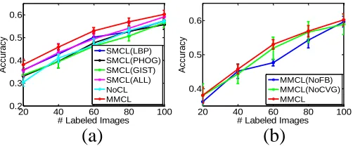
Fig. 2. Validations of our MMCL motivation. (a) compares the performance of multi-modal curriculum learning with single-modal curriculum learning and plain learning; (b) shows the effects of some key steps in our MMCL model.
256-dimensional Local Binary Patterns (LBP) [48] features. Therefore, three different modalities are formed to serve as the input of all the compared methods. Note that these feature descriptors are histogram-based and every element in a feature vector falls into [0,1], so none of them will dominate the learning performance.
A. Algorithm Validation
Firstly, we use a subset of the Caltech256 dataset [49] to demonstrate two arguments: 1) curriculum learning is critical to improving classification performance, and 2) MMCL is superior to single-modal curriculum learning (SMCL). The images of dog, goose, swan and zebra in Caltech256 are employed, and each type of animals contains 80 examples. For MMCL, each feature constitutes a modality, and Algo-rithm 2 is utilized to accomplish the classification. We also report the results of SMCL, of which the model explained in Section III-A is adopted to handle each of the three feature descriptors (denoted “SMCL(LBP)”, “SMCL(PHOG)”, and “SMCL(GIST)”, respectively). Furthermore, we concatenate these three different feature vectors to a long vector, and apply SMCL again to simultaneously utilize the three fea-ture modalities (denoted “SMCL(ALL)”). At last, the plain learning model [11] in our algorithm is implemented based on the concatenated long feature vectors, to test the performance without curriculum learning (denoted “NoCL”).
We evaluate the classification accuracies of tested methods under different sizes of labeled set, and the experiment un-der each size is conducted ten times with different initially labeled images. The reported accuracies are then obtained by averaging over the outputs of these ten independent runs. Fig. 2(a) presents the result, in which the record under each number of labeled images includes mean accuracy as well as the standard deviation. It can be observed that MMCL and SMCL(ALL) always outperform NoCL under different numbers of labeled images, therefore the argument 1) above is verified. Specifically, SMCL(ALL) and MMCL outperform NoCL with the margins about 1%∼5% and 3%∼8%, respec-tively, therefore the effectiveness of curriculum learning has been demonstrated. Moreover, we see that MMCL achieves the highest record compared to all the other single-modal counterparts, which explicitly justifies the argument 2). It is also clearly shown that the concatenation of all different features (SMCL(ALL)) generally yields better performance
than simply working on a single feature (e.g.SMCL(PHOG), SMCL(LBP) and SMCL(GIST)). Therefore, properly exploit-ing different modalities for curriculum learnexploit-ing is superior to simply working on single modality. The reason lies in that multiple feature modalities convey richer image information than the single modality, and this is also consistent with our general understanding.
Next, we demonstrate the effectiveness of a number of key steps in our MMCL model, such as the establishment of learning feedback Eq. (17) and the convergence of propaga-tions Eq. (20). To demonstrate the contribution of learning feedback, we remove the feedback and fix the number of selected simplest images in each propagationttomin(20, b[t])
to generate the accuracy (see “MMCL(NoFB)” in Fig. 2(b)). To show the importance of converge, we plot the accuracy generated by the non-convergentF¯ (see “MMCL(NoCVG)”). By comparing the three curves in Fig. 2(b), we clearly see that performance decreases in the absence of each of the two manipulations. Therefore, incorporating these steps in our model contributes to improved accuracy.
Lastly, we visualize the curriculum images selected by our MMCL during the entire teaching and learning process. When the number of labeled images is 60, our MMCL takes totally 14 propagations to classify all the unlabeled images, and the selected simplest images under different iterations t are provided in Fig. 3. We can see that during the initial stage of the propagation, i.e. t= 1 ∼2, the teachers in MMCL tend to select the images containing complete objects with regular appearances. Besides, the backgrounds in these images are also generally clean and are very different from the foreground objects. When t = 8 ∼9, we see that some of the selected images only contain part of the objects (e.g. dog, goose and zebra), or reflect the objects with abnormal behavior compared to their normal conditions (e.g.swan). During the final stage of propagations, i.e. t = 11 ∼ 14, the curriculum examples are quite difficult because of the multiple crowded objects (e.g. dog, goose and zebra) or the uncommon observation angle (e.g.swan). Therefore, the introduced teachers in MMCL can accurately evaluate the difficulty level of every unlabeled image, and effectively organize the entire propagation process so that all the images are classified from simple to difficult.
B. Comparison with Other Methods
To further demonstrate the strength of the proposed method, we compare MMCL with other state-of-the-art algorithms on some typical image datasets.
Datasets. Eight image datasets with different contents are adopted for our experiments: CaltechAnimal [49] for animal classification, Architecture [50] for architecture style recognition, MSRC1 for natural image classification, UIUC
[51] for sports event recognition, Scene15 [52] for scene categorization,ORLFace2for face recognition, andCIFAR100
[53] and NUS-WIDE [54] for general image classification. Of these, CaltechAnimal is a subset ofCaltech256 consisted of nine different animals, and NUS-WIDEis formed by only
t
= 1
~
2
t
= 8
~
9
t
= 11
~
14
dog
goose
[image:9.612.54.564.53.183.2]swan
zebra
Fig. 3. The selected simplest images during the entire propagation process. It can be observed that the difficulty level of curriculum images gradually increases with the propagation proceeds.
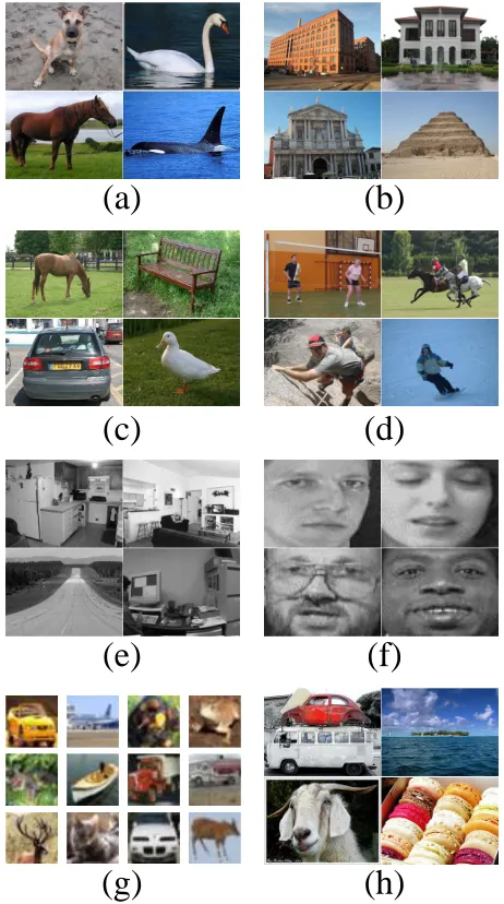
preserving the classes that have more than 100 images in the original dataset. The details of these datasets are summarized in Table I. Besides, some example images of these datasets are provide in Fig. 5, which reflects that accurately classifying the images in these datasets is a very challenging task.
Baselines.Five semi-supervised image classifiers are adopted for comparison. The Gaussian Field and Harmonic Functions (GFHF) [11] is a classical SSL algorithm, which also serves as the learner in our proposed methodology. Dynamic Label Propagation (DLP) [8] is a recently proposed single-modal semi-supervised image classifier. For multi-modal baselines, Adaptive Multi-Modal Semi-Supervised classifier (AMMSS) [1] and Sparse Multiple Graph Integration (SMGI) [55] are employed for comparison as they also operate on multiple graphs. The results of SMCL introduced in Section III-A are also reported. Among the compared existing methods, the codes of AMMSS and SMGI are directly provided by the authors. We implement GFHF and DLP by ourselves because both methods can be easily reproduced in lines of MATLAB code.
As explained at the beginning of Section IV, GIST, LBP and PHOG features constitute three modalities for the multi-modal algorithms such as AMMSS, SMGI and our MMCL. These three descriptors are concatenated into a long feature vector for single-modal methodologies including GFHF, DLP and SMCL.
Experimental settings. Similar to Section IV-A, the accu-racies of all the algorithms are evaluated under different selections of initially labeled images, and at least one labeled image is selected in each class. The reported accuracies and standard deviations are calculated as the mean value of the outputs of ten independent runs.
To achieve fair comparison, the identical 10-NN graphs are built via adaptive edge weighting [38] for all the methods except DLP. In DLP, the 10-NN graph is built by leveraging the Gaussian kernel as required. The key parameters in SMGI are optimally tuned toλ1= 0.01andλ2= 0.1via searching the
grid{0.01,0.1,1,10}, andrandλin AMMSS are respectively set to 0.5 and 10. As recommended by the authors, we adjust αandλin DLP to 0.05 and 0.1 throughout the experiments. Results & Analyses. The experimental results on the eight datasets are shown in Fig. 4. Figs. 4 (a)∼(h) indicate that
(a)
(b)
(c)
(d)
(f)
(e)
(h)
(g)
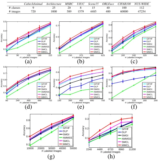
[image:9.612.322.553.258.672.2]TABLE I
AN OVERVIEW OF ADOPTED DATASETS.
CaltechAnimal Architecture MSRC UIUC Scene15 ORLFace CIFAR100 NUS-WIDE
# classes 9 25 20 8 15 40 100 112
# images 720 1000 589 1579 4485 400 60000 47254
45 90 135 180 225
0.2 0.3 0.4 0.5
# Labeled Images
Ac
c
urac
y
GFHF DLP SMGI AMMSS SMCL MMCL
80 240 400 560 720
0.4 0.5 0.6 0.7 0.8
# Labeled Images
Ac
c
urac
y
GFHF DLP SMGI AMMSS SMCL MMCL
150 300 450 600 750
0.3 0.4 0.5 0.6
# Labeled Images
Ac
c
urac
y
GFHF DLP SMGI AMMSS SMCL MMCL
(a)
(b)
(e)
(d)
40 80 120 160 200
0.5 0.6 0.7 0.8 0.9 1
# Labeled Images
Ac
c
urac
y
GFHF DLP SMGI AMMSS SMCL MMCL
(c)
(f)
125 250 375 500 625
0.3 0.5 0.7
# Labeled Images
Ac
c
urac
y
GFHF DLP SMGI AMMSS SMCL MMCL
80 160 240 320 400
0.4 0.5 0.6 0.7 0.8
# Labeled Images
Ac
c
urac
y
GFHF DLP SMGI AMMSS SMCL MMCL
(g)
(h)
10000 20000 30000 40000 50000
0.2 0.4 0.6 0.8
# Labeled Images
Ac
c
urac
y
GFHF DLP SMGI AMMSS SMCL MMCL
2240 4480 6720 8960 11200
0.1 0.2 0.3
# Labeled Images
Ac
c
urac
y
GFHF DLP SMGI AMMSS SMCL MMCL
Fig. 4. Comparison of MMCL with other baselines on eight image datasets. (a) isCaltechAnimaldataset, (b) isArchitecturedataset, (c) isMSRCdataset, (d) isUIUCdataset, (e) isScene15dataset, (f) isORLFacedataset, (g) isCIFAR100dataset, and (h) isNUS-WIDEdataset.
the proposed MMCL achieves the highest accuracy on the datasetsCaltechAnimal,Architecture,MSRC,UIUC,Scene15,
CIFAR100andNUS-WIDE. Numerically, MMCL leads SMCL with the margins approximately 2%, 3%, 3%, 3%, 4%, 4%, and 4% on the above seven datasets, respectively, and also significantly outperforms the best existing method SMGI or GFHF with the margins 3%, 3%, 4%, 4%, 4%, 5% and 5%, accordingly. On theORLFace dataset revealed by Fig. 4
(f), MMCL performs better than SMGI when the number of labeled images ranges from 40 to 160. MMCL is slightly surpassed by SMGI when the size of labeled set is 200. Furthermore, we observe that on all the datasets the standard deviations of MMCL are very small, suggesting that MMCL is insensitive to the selection of initially labeled examples.
GFHF
DLP
SMGI
AMMSS
SMCL
MMCL
Bicycle Chair Croquet Individual 28
Fig. 6. Classification results of the compared methods on several visually challenging images. The red crosses represent “incorrect classifications” while the green ticks denote “correct classifications”.
favorably compared to the other single-modal methods such as DLP (blue curve) and GFHF (cyan curve). MMCL (red curve) generally achieves better performance than other multi-modal approaches like SMGI (black curve) and AMMSS (green curve). Therefore, the established curriculums does help to optimize the learning process and generate encouraging classification performance. Secondly, sometimes the accuracy improvement brought by SMCL over GFHF is very marginal, such as on Architecture, UIUC, Scene15, ORLFace, and CI-FAR100datasets. Comparatively, MMCL is significantly better than GFHF, and also enhances the performance of SMCL on all the datasets. Therefore, generating curriculums from multiple modalities is superior to only employing a single modality consisted of a long concatenated feature vector. This reflects that directly putting different types of features into a long vector is not an ideal way to handle multi-modal cases. The information from different sources should instead be integrated in an informed way, such that the strength of every modality can be fully exploited. These observations also comply with our findings in Section IV-A and again demonstrate the validity of the two arguments therein. Further insight. As mentioned in the Introduction, MMCL can achieve higher classification due to its strong ability for handling difficult images. To illustrate this point, we investi-gate the classification correctness of the compared methods on some difficult images in the adopted datasets (see Fig. 6). In the “Bicycle” image, the occlusion and overlapping of bicycles make classification very difficult. The image belonging to “Chair” category contains one table and multiple chairs. The two men in the “Croquet” image are very small, and identi-fying their activities is nontrivial. The person in “Individual 28” wears a pair of glasses, which poses a great difficulty for accurate face recognition. Though these example images are visually challenging, MMCL is able to assign them the correct labels, whereas other methods fail to accurately classifying all these images with the identical initially labeled images. Therefore we conclude that multi-modal curriculum learning is beneficial to ease the learning on complicated visual concepts.
C. Parametric Sensitivity
The weighting factor β and initial learning rate γ are two tuning parameters in our MMCL algorithm. This section
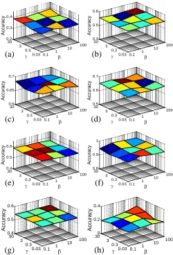
[image:11.612.313.563.55.423.2]stud-0.1 1 10 100 0.03 0.3 3 30 0.4 0.5 0.6 A ccu ra cy 0.1 1 10 100 0.03 0.3 3 30 0.2 0.3 0.4 A ccu ra cy
(a)
(b)
0.1 1 10 100 0.03 0.3 3 30 0.5 0.6 0.7 A ccu ra cy 0.1 1 10 100 0.03 0.3 3 30 0.8 0.9 1 A ccu ra cy(d)
(f)
0.1 1 10 100 0.03 0.3 3 30 0.6 0.65 0.7 A ccu ra cy(c)
0.1 1 10 100 0.03 0.3 3 30 0.4 0.5 0.6 A ccu ra cy(e)
0.1 1 10 100 0.03 0.3 3 300 0.2 0.4 A ccu ra cy(h)
0.1 1 10 100 0.03 0.3 3 30 0.4 0.5 0.6 A ccu ra cy(g)
Fig. 7. Parametric sensitivity of MMCL w.r.t.βandγ. (a) isCaltechAnimal dataset, (b) isArchitecturedataset, (c) isMSRCdataset, (d) isUIUCdataset, (e) isScene15dataset, (f) isORLFacedataset, (g) isCIFAR100dataset, and (h) isNUS-WIDEdataset.
ies how their variations influence the output accuracy. To this end, we fix the numbers of labeled images in the above eight datasetsCaltechAnimal,Architecture,MSRC,UIUC,Scene15,
ORLFace,CIFAR100,NUS-WIDEto 135, 375, 240, 400, 450, 120, 30000, 6720, respectively, and change β and γ to see the produced classification accuracy. The experimental results are illustrated in Fig. 7. It can be observed that even though β andγcover wide ranges (β∈[0.1,100]andγ∈[0.03,30]), the accuracies remain substantially unchanged, suggesting that the model output is very robust to the variations of these tuning parameters. As a result, the parameters incorporated by MMCL can be easily adjusted. Besides, MMCL is shown to achieve satisfactory performance overall on all datasets when β= 10 andγ= 3, which explains the reason that we choose this parameter setting for our experiments.
V. CONCLUSION
[image:11.612.47.300.55.186.2]different feature modalities is properly exploited and integrat-ed, based on which a curriculum learning sequence (i.e., a sequence for classifying unlabeled images) is generated in a simple-to-difficult order. Through extensive experiments, we demonstrated the superiority of the proposed multi-modal curriculum learning over the state-of-the-arts in terms of semi-supervised image classification accuracy. We also found that our approach is general in nature and hence readily applicable to other semi-supervised classification problems. In the future, we plan to extend MMCL to dealing with the noisy label cases [56], in which the labeled images with potentially incorrect labels are difficult and should be re-classified in later propagations.
REFERENCES
[1] X. Cai, F. Nie, W. Cai, and H. Huang, “Heterogeneous image features in-tegration via multi-modal semi-supervised learning model,” inComputer Vision (ICCV), IEEE International Conference on, 2013, pp. 1737–1744. [2] D. Dai and L. Gool, “Ensemble projection for semi-supervised image classification,” inComputer Vision (ICCV), IEEE International Confer-ence on, 2013, pp. 2072–2079.
[3] R. Fergus, Y. Weiss, and A. Torralba, “Semi-supervised learning in gi-gantic image collections,” inAdvances in Neural Information Processing Systems (NIPS), 2009, pp. 522–530.
[4] M. Guillaumin, J. Verbeek, and C. Schmid, “Multimodal semi-supervised learning for image classification,” inComputer Vision and Pattern Recognition (CVPR), IEEE Conference on, 2010, pp. 902–909. [5] Y. Luo, D. Tao, B. Geng, C. Xu, and S. Maybank, “Manifold regularized multitask learning for semi-supervised multilabel image classification,” Image Processing, IEEE Transactions on, vol. 22, no. 2, pp. 523–536, 2013.
[6] L. Jing and M. Ng, “Sparse label-indicator optimization methods for image classification,”Image Processing, IEEE Transactions on, vol. 23, no. 3, pp. 1002–1014, 2014.
[7] X. Liu, T. Guo, L. He, and X. Yang, “A low-rank approximation-based transductive support tensor machine for semisupervised classification,” Image Processing, IEEE Transactions on, vol. 24, no. 6, pp. 1825–1838, 2015.
[8] B. Wang, Z. Tu, and J. Tsotsos, “Dynamic label propagation for semi-supervised multi-class multi-label classification,” inComputer Vision (ICCV), IEEE International Conference on, 2013, pp. 425–432. [9] W. Xie, Z. Lu, Y. Peng, and J. Xiao, “Graph-based multimodal
semi-supervised image classification,” Neurocomputing, vol. 138, pp. 167– 179, 2014.
[10] Y. Bengio, J. Louradour, R. Collobert, and J. Weston, “Curriculum learning,” in Proc. International Conference on Machine Learning (ICML), 2009, pp. 41–48.
[11] X. Zhu and Z. Ghahramani, “Learning from labeled and unlabeled data with label propagation,” CMU-CALD-02-107, Tech. Rep., 2002. [12] X. Zhu and B. Goldberg, Introduction to Semi-Supervised Learning.
Morgan & Claypool Publishers, 2009.
[13] C. Rosenberg, M. Hebert, and H. Schneiderman, “Semi-supervised self-training of object detection models,” in IEEE Winter Conference on Applications of Computer Vision (WACV), 2005.
[14] T. Joachims, “Transductive inference for text classification using sup-port vector machines,” inProc. International Conference on Machine Learning (ICML), 1999, pp. 200–209.
[15] Y. Li and Z. Zhou, “Towards making unlabeled data never hurt,” in Proc. International Conference on Machine Learning (ICML), 2011, pp. 1081–1088.
[16] Y. Wang and S. Chen, “Safety-aware semi-supervised classification,” Neural Networks and Learning Systems, IEEE Transactions on, vol. 24, no. 11, pp. 1763–1772, 2013.
[17] M. Belkin, P. Niyogi, and V. Sindhwani, “Manifold regularization: A geometric framework for learning from labeled and unlabeled examples,” The Journal of Machine Learning Research, vol. 7, pp. 2399–2434, 2006.
[18] X. Zhu, Z. Ghahramani, and J. Lafferty, “Semi-supervised learning using Gaussian fields and harmonic functions,” inProc. International Conference on Machine Learning (ICML), 2003, pp. 912–919.
[19] C. Gong, D. Tao, K. Fu, and J. Yang, “Fick’s law assisted propagation for semisupervised learning,”Neural Networks and Learning Systems, IEEE Transactions on, vol. 26, no. 9, pp. 2148–2162, 2015.
[20] A. Shrivastava, S. Singh, and A. Gupta, “Constrained semi-supervised learning using attributes and comparative attributes,” inEuropean Con-ference on Computer Vision (ECCV), 2012, pp. 369–383.
[21] A. Mahmood, A. Mian, and R. Owens, “Semi-supervised spectral clustering for image set classification,” inComputer Vision and Pattern Recognition (CVPR), IEEE Conference on, 2014, pp. 121–128. [22] G. Valls, T. Bandos, and D. Zhou, “Semi-supervised graph-based
hy-perspectral image classification,”Geoscience and Remote Sensing, IEEE Transactions on, vol. 45, no. 10, pp. 3044–3054, 2007.
[23] C. Xu, T. Liu, D. Tao, and C. Xu, “Local rademacher complexity for multi-label learning,”Image Processing, IEEE Transactions on, vol. 25, no. 3, pp. 1495–1507, 2016.
[24] C. Xu, D. Tao, and C. Xu, “A survey on multi-view learning,” arX-iv:1304.5634, 2013.
[25] A. Blum and T. Mitchell, “Combining labeled and unlabeled data with co-training,” in Proc. Conference on Computational learning theory, 1998, pp. 92–100.
[26] C. Ding and D. Tao, “Robust face recognition via multimodal deep face representation,”Multimedia, IEEE Transactions on, vol. 17, no. 11, pp. 2049–2058, 2015.
[27] G. Lanckriet, N. Cristianini, P. Bartlett, L. Ghaoui, and M. Jordan, “Learning the kernel matrix with semidefinite programming,”The Jour-nal of Machine Learning Research, vol. 5, pp. 27–72, 2004.
[28] M. White, X. Zhang, D. Schuurmans, and Y. Yu, “Convex multi-view subspace learning,” inAdvances in Neural Information Processing Systems (NIPS), 2012, pp. 1673–1681.
[29] Y. Luo, T. Liu, D. Tao, and C. Xu, “Multiview matrix completion for multilabel image classification,”Image Processing, IEEE Transactions on, vol. 24, no. 8, pp. 2355–2368, 2015.
[30] M. Kumar, B. Packer, and D. Koller, “Self-paced learning for latent variable models,” inAdvances in Neural Information Processing Systems (NIPS), 2010, pp. 1189–1197.
[31] L. Jiang, D. Meng, S. Yu, Z. Lan, S. Shan, and A. Hauptmann, “Self-paced learning with diversity,” inAdvances in Neural Information Processing Systems (NIPS), 2014, pp. 2078–2086.
[32] L. Jiang, D. Meng, Q. Zhao, S. Shan, and A. Hauptmann, “Self-paced curriculum learning,” in AAAI Conference on Artificial Intelligence (AAAI), 2015.
[33] C. Gong, D. Tao, W. Liu, L. Liu, and J. Yang, “Label propagation via teaching-to-learn and learning-to-teach,”Neural Networks and Learning Systems, IEEE Transactions on, 2016.
[34] C. Gong, D. Tao, J. Yang, and W. Liu, “Teaching-to-learn and learning-to-teach for multi-label propagation,” inAAAI Conference on Artificial Intelligence (AAAI), 2016.
[35] Y. Lee and K. Grauman, “Learning the easy things first: Self-paced visual category discovery,” inComputer Vision and Pattern Recognition (CVPR), IEEE Conference on, 2011, pp. 1721–1728.
[36] J. Supancic and D. Ramanan, “Self-paced learning for long-term tracking,” inComputer Vision and Pattern Recognition (CVPR), IEEE Conference on, 2013, pp. 2379–2386.
[37] L. Jiang, D. Meng, T. Mitamura, and A. Hauptmann, “Easy samples first: self-paced reranking for zero-example multimedia search,” inACM Multimedia Conference (ACM MM), 2014, pp. 547–556.
[38] M. Karasuyama and H. Mamitsuka, “Manifold-based similarity adapta-tion for label propagaadapta-tion,” inAdvances in Neural Information Process-ing Systems (NIPS), 2013, pp. 1547–1555.
[39] X. Zhu, J. Lafferty, and Z. Ghahramani, “Semi-supervised learning: From Gaussian fields to Gaussian processes,” CMU-CS-03-175, Tech. Rep., 2003.
[40] C. Bishop,Pattern recognition and machine learning. springer, 2006. [41] H. Qiu and E. Hancock, “Clustering and embedding using commute times,” Pattern Analysis and Machine Intelligence, IEEE Transactions on, vol. 29, no. 11, pp. 1873–1890, 2007.
[42] D. Bertsekas,Constrained optimization and Lagrange multiplier meth-ods. Academic press, 2014.
[43] P. Absil and J. Malick, “Projection-like retractions on matrix manifolds,” SIAM Journal on Optimization, vol. 22, no. 1, pp. 135–158, 2012. [44] F. Pompili, N. Gillis, P. Absil, and F. Glineur, “Two algorithms for
or-thogonal nonnegative matrix factorization with application to clustering,” arXiv:1201.0901v2, 2014.
[46] A. Bosch, A. Zisserman, and X. Munoz, “Representing shape with a spatial pyramid kernel,” inProceedings of the 6th ACM international conference on Image and video retrieval. ACM, 2007, pp. 401–408. [47] A. Oliva and A. Torralba, “Modeling the shape of the scene: A
holistic representation of the spatial envelope,”International Journal of Computer Vision, vol. 42, no. 3, pp. 145–175, 2001.
[48] T. Ahonen, A. Hadid, and M. Pietik¨ainen, “Face recognition with local binary patterns,” inEuropean Conference on Computer Vision (ECCV). Springer, 2004, pp. 469–481.
[49] G. Griffin, A. Holub, and P. Perona, “Caltech-256 object category dataset,” 2007.
[50] Z. Xu, Z. Hong, Y. Zhang, J. Wu, A. Tsoi, and D. Tao, “Multinomial latent logistic regression for image understanding,”Image Processing, IEEE Transactions on, vol. 25, no. 2, pp. 973–987, 2016.
[51] L. Li and F. Li, “What, where and who? classifying events by scene and object recognition,” inComputer Vision (ICCV), IEEE International Conference on, 2007, pp. 1–8.
[52] S. Lazebnik, C. Schmid, and J. Ponce, “Beyond bags of features: Spatial pyramid matching for recognizing natural scene categories,” in Computer Vision and Pattern Recognition (CVPR), IEEE Conference on, 2006, pp. 2169–2178.
[53] A. Krizhevsky and G. Hinton, “Learning multiple layers of features from tiny images,” U. Toronto, Tech. Rep., 2009.
[54] T. Chua, J. Tang, R. Hong, H. Li, Z. Luo, and Y. Zheng, “Nus-wide: a real-world web image database from national university of singapore,” inProceedings of the ACM international conference on image and video retrieval. ACM, 2009, pp. 48–56.
[55] M. Karasuyama and H. Mamitsuka, “Multiple graph label propagation by sparse integration,”Neural Networks and Learning Systems, IEEE Transactions on, vol. 24, no. 12, pp. 1999–2012, 2013.
[56] T. Liu and D. Tao, “Classification with noisy labels by importance reweighting,”Pattern Analysis and Machine Intelligence, IEEE Trans-actions on, vol. 38, no. 3, pp. 447–461, 2016.
Chen Gongreceived his bachelor degree from East China University of Science and Technology (E-CUST) in 2010. Currently he is a dual doctorial de-gree student at the Institute of Image Processing and Pattern Recognition, Shanghai Jiao Tong University (SJTU), and the Centre for Quantum Computation & Intelligent Systems, University of Technology Sydney (UTS), under the supervision of Prof. Jie Yang and Prof. Dacheng Tao. His research interests mainly include machine learning, data mining and learning-based vision problems. He has published 28 technical papers at prominent journals and conferences such as IEEE T-NNLS, IEEE T-IP, IEEE T-CYB, CVPR, AAAI, ICME, etc. He received the “National Scholarship” awarded by the Ministry of Education in 2013 and 2014, the “Excellent Self-financed Overseas Student Scholarship” awarded by China Scholarship Council in 2015, and the “IBM Excellent Student Scholarship” in 2015.
Dacheng Tao(F’15) is Professor of Computer Sci-ence with the Centre for Quantum Computation & Intelligent Systems, and the Faculty of Engineering and Information Technology in the University of Technology Sydney. He mainly applies statistics and mathematics to data analytics problems and his research interests spread across computer vision, data science, image processing, machine learning, and video surveillance. His research results have expounded in one monograph and 200+ publications at prestigious journals and prominent conferences, such as IEEE T-PAMI, T-NNLS, T-IP, JMLR, IJCV, NIPS, ICML, CVPR, ICCV, ECCV, AISTATS, ICDM; and ACM SIGKDD, with several best paper awards, such as the best theory/algorithm paper runner up award in IEEE ICDM’07, the best student paper award in IEEE ICDM’13, and the 2014 ICDM 10-year highest-impact paper award. He received the 2015 Australian Scopus-Eureka Prize, the 2015 ACS Gold Disruptor Award and the UTS Vice-Chancellor’s Medal for Exceptional Research. He is a Fellow of the IEEE, OSA, IAPR and SPIE.
Stephen J. Maybank(F’11) received the BA degree in mathematics from King’s College Cambridge in 1976 and the PhD degree in computer science from Birkbeck College, University of London in 1988. He was a research scientist at GEC from 1980 to 1995, first at MCCS, Frimley, and then, from 1989, at the GEC Marconi Hirst Research Centre in London. In 1995 he became a lecturer in the Department of Computer Science at the University of Reading and in 2004 he became a professor in the Department of Computer Science and Information Systems at Birkbeck College, University of London. His research interests include camera calibration, visual surveillance, tracking, filtering, applications of projective geometry to computer vision and applications of probability, statistics and information theory to computer vision. Maybank is the author or co-author of more than 160 scientific publications and one book. He is a Fellow of the IEEE and a Fellow of the Royal Statistical Society. He received the Koenderink Prize in 2008.
Wei Liu (M’14) received the Ph.D. degree from Columbia University, New York, NY, USA, in 2012. He was a recipient of the 2013 Jury Award for Best Thesis of Columbia University. He has been a research staff member of IBM T. J. Watson Research Center, Yorktown Heights, NY, USA since 2012. His research interests include machine learning, big data analytics, computer vision, pattern recognition, and information retrieval.
IEEE TRANSACTIONS ON IMAGE PROCESSING 13