BIROn - Birkbeck Institutional Research Online
Fenner, Trevor and Levene, Mark and Loizou, George (2015) A stochastic
evolutionary model for capturing human dynamics.
Journal of Statistical
Mechanics: Theory and Experiment (JSTAT) 2015 , ISSN 1742-5468.
Downloaded from:
Usage Guidelines:
Please refer to usage guidelines at or alternatively
arXiv:1502.07558v3 [physics.soc-ph] 21 Aug 2015
A stochastic evolutionary model for capturing human dynamics
Trevor Fenner, Mark Levene, and George Loizou Department of Computer Science and Information Systems
Birkbeck, University of London London WC1E 7HX, U.K. {trevor,mark,george}@dcs.bbk.ac.uk
Abstract
The recent interest in human dynamics has led researchers to investigate the stochastic processes that explain human behaviour in various contexts. Here we propose a generative model to capture the dynamics of survival analysis, traditionally employed in clinical trials and reliability analysis in engineering. We derive a general solution for the model in the form of a product, and then a continuous approximation to the solution via the renewal equation describing age-structured population dynamics. This enables us to model a wide range of survival distributions, according to the choice of the mortality distribution. We provide empirical evidence for the validity of the model from a longitudinal data set of popular search engine queries over 114 months, showing that the survival function of these queries is closely matched by the solution for our model with power-law mortality.
Keywords: human dynamics, generative model, survival analysis, power-law mortality, Weibull distribution
1
Introduction
Recent interest in complex systems, such as social networks, the world-wide-web, email net-works and mobile phone netnet-works [Bar07], has led researchers to investigate the processes that could explain the dynamics of human behaviour within these networks. Barab´asi [Bar05] suggested that the bursty nature of human behaviour, for example, when measuring the inter-event response time of email communication, is a result of a decision-based queuing process. In particular, humans tend to prioritise actions, for example, when deciding which email to respond to, and therefore a priority queue model was proposed in [Bar05], leading to a heavy-tailed power-law distribution of inter-event times. The availability of large data sets, such as mobile phone records, has widened the applicability of human dynamics investigation, for example, in an attempt by Schneider et al. [SBCG13] to uncover the characteristics of daily mobility patterns. Human dynamics is not limited to the study of behaviour within communication networks, as can be seen, for example, by a recent proposal of Mitnitski et al. [MSR13], who apply a simple stochastic queueing model to the complex phenomenon of aging in order to illustrate how health deficits accumulate with age.
work or to recover from a disease. In the context of email communication mentioned above, an event might be a reply to an email. Traditional applications of survival analysis are in clinical trials [FL00], and in understanding the mechanisms in biological ageing [GG01]. The methods used in survival analysis overlap with those used in engineering for reliability life data analysis [OK12]. Reliability engineering has many applications, for example, in manufacturing processes, and in software design and testing. However, one can envisage that survival analysis would find application in newer human dynamics scenarios in complex systems, such as those arising in social and communication networks [Bar05, CGW+
08, MAAJ13].
Of particular interest to us has been the formulation of a generative model in the form of a stochastic process by which a complex system evolves and gives rise to a power law or other distribution [FLL07, FLL12]. This type of research builds on the early work of Simon [Sim55], and the more recent work of Barab´asi’s group [AB02] and other researchers [BSV07]. In the context of human dynamics, the priority queue model [Bar05] mentioned above is a generative model characterised by a heavy-tailed distribution.
In the bigger picture, one can view the goal of such research as being similar to that of
social mechanisms [HS98], which looks into the processes, or mechanisms, that can explain observed social phenomena. Using an example given in [Sch98], the growth in the sales of a book can be explained by the well-known logistic growth model [TW02], and more recently we have shown that the process of conference registration with an early bird deadline can be modelled by bi-logistic growth [FLL13]. Such research can also be grounded within the field of sociophysics [Gal08, CFL09], which applies methods from physics to explain social phenomena such as opinion dynamics. Critical phenomena are important here, where a transition to global behaviour emerges from the interactions of many individuals. The individuals may be neurons as in [LAE+12], where criticality emerges as neuron cooperation, or people’s decisions as in [PS10], where the popularity of movies emerges as collective choice behaviour.
In [FLL14] we proposed a simple generative model to capture the essential dynamics of survival analysis applications. For this purpose, we make use of an urn-based stochastic model, where theactorsare calledballs, and a ball being present inurni, theith urn, indicates
that the actor represented by the ball has so far survived for i time steps. An actor could, for example, be a subject in a clinical trial, an email that has not yet been replied to, or an ongoing phone call. As a simplification, we assume that time is discrete and that, at any given time, one ball may join the system with a fixed birth probability. Alternatively, with a fixed probability, an existing ball in the system may be chosen uniformly at random and discarded, i.e. a mortality(or death) event occurs. It is evident that, at any given time, say
t, we may have at most one ball in urni, for alli≤t.
The main result in [FLL14] was to derive a power-law distribution for the probability that, after tsteps of the stochastic process outlined above, there is a surviving ball in urni. Thus,
in our model, the survival function[KK12], which gives the probability that an actor (in our model, a ball) survives for more than a given time, can be approximated by a power-law distribution. It is interesting to observe that the resulting distribution has two parameters,
i and t, as in [FLL12], whereas most previously studied generative stochastic models [AB02, New05], including those in our previous work, for example [FLL07], result in steady state distributions that are asymptotic in t to a distribution with a single parameteri.
when mortality follows a power-law distribution. Our model can be described by a difference equation that has an explicit solution in the form of a product. The difference equation can be approximated by a partial differential equation that coincides with the renewal equation from age-structured population dynamics with a constant birth rate [Cha94, LB08]. More specifically, we show that, by choosing the appropriate mortality distribution, the survival distribution of actors will follow an exponential, power-law or Weibull distribution. The Weibull distribution [Rin09] is of particular interest due to its prevalence in modelling life data(also known as survival data, time to event data, or time to failure data) [KK12, OK12]. It also has application in the instance theory of automaticity [Col95], where it is argued that the retrieval time of traces from memory follow a Weibull distribution, and more recently as a model for Internet response times [CM06], where it is shown to be a better fit to the data than a power-law distribution. We provide empirical evidence for the validity of the model from a longitudinal data set of popular search engine queries over 114 months, showing that the survival function of these queries closely follows the distribution generated by our model. The rest of the paper is organised as follows. In Section 2, we present our stochastic urn-based model that provides us with a mechanism to model the essential dynamics of survival models. We then derive a difference equation to describe the process and obtain its solution in the form of a product. In Section 3, we provide a continuous approximation to the model, which has a solution in the form of an integral. In Section 4, we derive the resulting distributions in the continuous case for several mortality distributions; in particular, when the mortality distribution is a power law, we obtain a Weibull distribution. In Section 5, we apply our generative model to the survival of popular search engine queries posted on Google Trends (www.google.com/trends/hottrends). Finally, in Section 6, we give our concluding remarks.
2
An Evolutionary Urn Transfer Model
In this section we formalise a stochastic urn model that allows us to model the dynamic aspects of a complex system, and then present the difference equations that describe the model. This model is a direct extension of the one introduced in [FLL14], in that it caters for an arbitrary mortality distribution.
We assume a countable number of urns, urn0, urn1, . . . , where a ball (or actor) in urni
is said to be ofage i. Initially, all the urns are empty. We define a stochastic process [Ros96] where, at any timet,t≥1, a new ball may bebornby inserting it intourn0, and an existing ball of age ican die by being discarded fromurni, for all i >0.
For a given age i and time t, we let µ(i, t) be the probability that a ball in urni dies at
time t; µ(i, t) is known as the mortality distribution. We always require that µ(0, t) = 0 for all t. Finally, urni is empty when i > t.
At timet, the stochastic process then proceeds as follows in order to obtain the configu-ration at time t+ 1, wheret≥1.
(i) For eachi, 0≤i≤t, ifurni is non-empty then, with probabilityµ(i, t), the ball inurni
is discarded.
(ii) Next, the ages of all balls remaining in the system are incremented by 1, i.e. a ball in
(iii) Finally, with probabilityp, where 0< p <1, a birth occurs, i.e. a ball is inserted into
urn0.
We now letF(i, t)≥0 be a discrete function denoting the probability that there is a ball inurni at timet. Initially, we set F(0,0) =p andF(i,0) = 0 for all i >0.
The dynamics of the model can be captured by the following two equations:
F(0, t) =p for t≥0, (1) and
F(i+ 1, t+ 1) =F(i, t)−µ(i, t)F(i, t) for 0≤i≤t. (2)
We can expand (2) to obtain
F(i+ 1, t+ 1) =p
i Y
j=1
(1−µ(j, t−i+j)). (3)
3
A Stochastic Model Based on Population Dynamics
In this section, we present an approximate solution to the difference equation (2), by approxi-mating it by a first-order hyperbolic partial differential equation [Lax06]. This equation is the same as that used in age-structured models of population dynamics [Cha94]. We note that, in our model, the birth rate p is constant, rather than the more complex dynamics where the birth rate is determined by a distribution that depends on the ages of individuals and possibly on the timet.
We first rewrite (2) in the form:
F(i+ 1, t+ 1)−F(i+ 1, t) +F(i+ 1, t)−F(i, t) +µ(i, t)F(i, t) = 0, (4) and then approximate the discrete functionF(i, t) by a continuous functionf(i, t), withµ(i, t) now being a continuous density function. We then approximate
F(i+ 1, t+ 1)−F(i+ 1, t) by ∂f(i, t)
∂t
and
F(i+ 1, t)−F(i, t) by ∂f(i, t)
∂i .
From (4) we thus derive the first-order hyperbolic partial differential equation,
∂f(i, t)
∂t +
∂f(i, t)
∂i +µ(i, t)f(i, t) = 0. (5)
Note that, by (1),f(0, t) =pfor all t.
Equation (5) is the well-known transport equation in fluid dynamics [Lax06], and the
renewal equation in population dynamics [PR91, Cha94, LB08]. Following Equation 1.22 in [Cha94], the solution of (5), when i≤t, is given by
f(i, t) =f(0, t−i) exp
−
Z i
0
µ(i−s, t−s)ds
4
Choosing the mortality distribution
In this section, we make use of the generality of our model by investigating four special cases of the mortality distribution. We note thatµ(i, t) can be viewed as adiscrete hazard function
[BG03], denoting the conditional probability that an actor of ageifails at timet, given that this actor did not fail previously.
In Subsection 4.1, we look at the case when the mortality distribution is constant. In Subsection 4.2, we look at the case when the mortality distribution is independent of age. In Subsection 4.3, we look at the case when the mortality distribution is preferential. Finally, in Subsection 4.4, we look at the case when the mortality distribution is a power law in the age of the actor.
4.1 Constant mortality
In the simplest case, we let
µ(i, t) =C, (7) for i >0 and some positive constant C.
Substituting this into (6) and using the boundary condition (1), we obtain
f(i, t) =pexp (−Ci),
which is the survival function of the exponential distribution, with rate parameterC.
4.2 Age-independent mortality
Let
µ(i, t) =µ(t) = κ
t, (8)
for i >0 and some positive constantκ. In this case mortality does not depend oni, the age of the actor, so all actors who are alive at time tare equally likely to die.
Substituting (8) into (6), we obtain
f(i, t) =pexp
−
Z i
0
κ t−s
ds
=pexp
κln
t−i t
=p
1− i
t
κ
,
which is a power-law distribution in (t−i)/t, as was derived from first principles in [FLL14].
4.3 Preferential mortality
Let
µ(i, t) = κi
t2, (9)
note that preferential mortality, being proportional to the agei, has some resemblance to the preferential attachment rule in evolving networks [AB02], where the probability that a node (or actor) gains a new link is proportional to the number of links it already has.
Substituting (9) into (6) we obtain
f(i, t) =pexp
−
Z i
0
κ(i−s) (t−s)2
ds
=pexp
−κ ln t t−i
− i
t
=pexp
κi
t 1− i t
κ
,
which is a power-law distribution with an exponential correction.
4.4 Power-law mortality
Let
µ(i, t) =µ(i) =λ(1 +ρ)iρ, (10) fori > 0, and some shape parameter ρ, −1 ≤ρ ≤ 0, and scale parameter λ > 0. We note that, in this case, mortality is time invariant.
Substituting (10) into (6) we obtain
f(i, t) =pexp
−
Z i
0
λ(1 +ρ) (i−s)ρ
ds
=pexp −λ i1+ρ
, (11)
which, when divided by p, is the survival function of the Weibull distribution [Rin09], also known as the stretched exponential function [LS98]. (We note that our definition of the scale parameter is slightly different from that given in [Rin09].) The Weibull distribution is widely used in survival models [KK12] and reliability engineering [OK12], and it is therefore important to be able to model it.
Inspecting (10), we note that, in our model, the probability of mortality decreases with age. The survival probabilityf(i, t) also decreases with age, and decreases faster for largerρ. We observe that this degenerates to the constant mortality case whenρ= 0, and that f(i, t) approaches a constant asρ gets close to −1.
Substituting (10) into (3), with k≥0, we obtain
F(i+ 1, t+ 1)
F(k, t+ 1) =
i Y
j=k
(1−λ(1 +ρ)jρ). (12)
Taking logarithms in (12) and using the approximation ln(1 +x) ≈ x, which holds for small x, we obtain
lnF(i+ 1, t+ 1)
F(k, t+ 1) ≈ −
i X
j=k
Using the first two correction terms of the Euler-Maclaurin summation formula [Apo99, Lam01] to approximate the right-hand side of (13) we obtain
i X
j=k
λ(1 +ρ)jρ≈ Z i
k
λ(1 +ρ)xρdx+ λ(1 +ρ) (i
ρ+kρ)
2 +
λ(1 +ρ)ρ iρ−1−kρ−1
12
=λ i1+ρ−k1+ρ
+λ(1 +ρ) (i
ρ+kρ)
2 +
λ(1 +ρ)ρ iρ−1−kρ−1
12 . (14)
Substituting (14) into (13) and rearranging, we obtain
−λi1+ρ≈ln
F(i+ 1, t+ 1
F(k, t+ 1)
−λk1+ρ+λ(1 +ρ) (iρ+kρ)
2 +
λ(1 +ρ)ρ iρ−1−kρ−1
12 . (15)
5
Application to the Survival of Popular Search Engine Queries
As mentioned in the introduction, survival analysis [KK12], dealing with the analysis of time-to-eventdata, is well established within the statistics community, and has many applications in disparate fields. In the context of human dynamics, survival analysis has recently been applied to large data sets. These include the analysis of phone call durations [VAFL10], the investigation of how long Wikipedia editors remain active [ZPL12], and the analysis of completion rates for students using intelligent tutoring systems [EB14].
In our model, the objects being monitored are represented by balls and they are considered to have survived for as long as they remain in the system. A death event is modelled by discarding a ball, and a birth event is modelled by inserting a new ball into the first urn. Our stochastic model has three input parameters: the birth probability p, the mortality distributionµ(i, t), and the timet at which the system is observed. Given these parameters, the survival probability of a ball inurni at timet, where i≤t, is approximated by f(i, t) as
given by (6), which depends on the form of the mortality distributionµ(i, t). In other words, givent,f(i, t) is the probability that a new ball enters the system at timet−iand survives for at leastisteps before it is discarded. In our empirical analysis below, we will make use of power-law mortality, which leads to the Weibull distribution, as in (11).
In survival analysis, we are often interested in the survival function S(θ) [KK12], which represents the probability that a patient in a given study survives for longer than a specified time θ. The survival function is usually estimated via a step function by computing the probability that a patient survives until timeθ, forθ= 1,2, . . . , t. This step function is known as theKaplan-Meier estimator [KM58, KK12]. By comparing (12), or the more general (3), with the Kaplan-Meier estimator for the survival function [KM58, equation (2b)], the latter is seen to be analogous toF(i, t) for an actor that was born at time t−i; more specifically,
S(i)≈F(i, t)/p.
We note that, although in theory the survival functionS(θ) does not depend on the length
The Kaplan-Meier estimator also takes into account censored data [KK12], when, for example, a patient drops out before the end of the study period. Although our evolutionary urn transfer model does not explicitly include censoring, it could be incorporated by allowing the possibility that when a ball is discarded it may be counted as either a death or censoring event. We further note that, while in traditional survival models patients join a study in batches, in our model individual balls continue to join the system with a fixed probability. Our model could be generalised to allow several balls to join the system at any given time, and also by letting the arrival probability p depend on t; we leave consideration of such enhancements for future work.
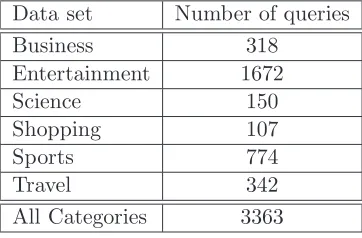
As a proof of concept for the model with power-law mortality, we analyse the survival of queries in the top-10 Google Trends “hot searches” (www.google.com/trends/hottrends). Data was collected monthly for the top-10 “hot searches” over 114 months from January 2004 until June 2013, for six categories (together with their subcategories in each case): Business & Politics (or simply Business), Entertainment, Nature & Science (or simply Science), Shopping & Fashion (or simply Shopping), Sports, and Travel & Leisure (or simply Travel). The number of distinct queries per category over the period is shown in Table 1. It is apparent from this statistic that the top-10 queries from Shopping change the least, while those from Entertainment change the most.
Data set Number of queries
Business 318
Entertainment 1672
Science 150
Shopping 107
Sports 774
Travel 342
[image:9.595.211.392.370.489.2]All Categories 3363
Table 1: Number of top-10 queries collected from Google Trends.
In this data set, the balls are top-10 queries, a death event occurs when a query leaves the top-10 in a given month, and a birth event occurs when a new query joins the top-10 in a given month (note that time is discrete and is measured in months). As we are examining power-law mortality, queries leave the top-10 according to (10). Thus, when ρ is non-zero, the probability of mortality decreases with age. As a result, a substantial number of queries are popular for a short duration, while the popularity of others lasts for much longer; we note that a similar observation, in the context of the popularity of movies, was made in [PS10]. Returning to our theme of human dynamics [CFL09], our stochastic urn model with power-law mortality contributes to a better understanding of collective phenomena, such as popularity, and how such global behaviour emerges from the decisions of individuals.
We first outline the methodology we have used to validate and evaluate our model, as-suming power-law mortality as in (10). We then give further details, before discussing and analysing the results.
of the product on the right-hand side of (12) fori= 1,2, . . . ,114, withk= 0, using the Kaplan-Meier estimates computed from the raw data.
(II) We use λ and ρ from (I) to compute, for each i, the product on the right-hand side of (12), with k= 0; we call this theproduct data. We then repeat the least-squares curve fitting using these values as a quick check that theλandρobtained are consistent with those from (I).
(III) Next we run simulations using the parametersλandρfrom (I), andp= 0.9. Using the averaged values of F(i, t) from the simulations, we again repeat the least-squares curve fitting, with k= 0, to obtain new values forλand ρ; these are compared to those from (I) for consistency.
(IV) We compute theDvalues from a Kolmogorov-Smirnov test to check whether the Kaplan-Meier estimates, the product data and the averaged simulation data are likely to have all come from the same distribution.
(V) Lastly, we adjust the averaged values of F(i, t) from the simulation using the Euler-Maclaurin correction, as on the right-hand side of (15), with k = 10 and the values of λand ρ obtained from step (III). We then use nonlinear regression to fit a Weibull distribution to the exponential of the adjusted estimates in (15). We compare theλand
ρ from this Weibull fit to those from (III), in order to check the plausibility of using the Weibull distribution as a continuous approximation to our model.
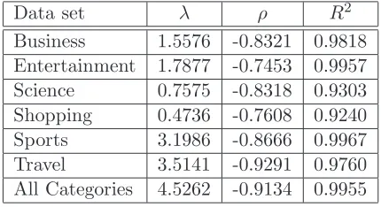
We first computed the Kaplan-Meier estimates from the raw data sets for the individual six categories and for their aggregation (All Categories). Recalling that the survival function
S(i) ≈F(i, t)/p, following (I), using Matlab we then obtained estimates for λ andρ by non-linear least-squares regression ofS(i) onifor fitting function (12), for i= 1,2, . . . ,114, with
k= 0. The estimated parametersλandρ are shown in the rows of Table 2, together with the coefficient of determination R2
[Mot95]; these show a very good fit for all of the categories. We observe that theR2
values for Science and Shopping are somewhat worse than the others, which could be attributed to the fact the number of queries in these categories is significantly smaller than the others, as can be seen from Table 1. Nonlinear least-squares curve fitting to the product data obtained using (12), as in (II), yields perfect fits, as expected.
Data set λ ρ R2
Business 1.5576 -0.8321 0.9818
Entertainment 1.7877 -0.7453 0.9957
Science 0.7575 -0.8318 0.9303
Shopping 0.4736 -0.7608 0.9240
Sports 3.1986 -0.8666 0.9967
Travel 3.5141 -0.9291 0.9760
[image:10.595.194.409.564.681.2]All Categories 4.5262 -0.9134 0.9955
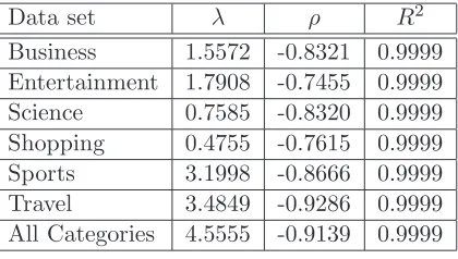
To test the validity of the model, as in (III), we then carried out simulations in Matlab of the stochastic urn transfer model using the values of λandρ shown in Table 2. We chose the valuep= 0.9 for all simulations, after running some sample simulations with other values of
p. The value of p is not critical since, as can be seen from (3), p is merely a scaling factor. The simulations were run for 114 steps, one for each month, for each of the categories, and these were repeated 105 times. For each category, we then calculated the average value of
F(i, t) fori= 1,2, . . . , t, over the 105
runs. The results of nonlinear least-squares curve fitting to these average values are shown in Table 3. Comparing Table 3 with Table 2 shows all the values of λand ρ to be very close.
To check the closeness between the Kaplan-Meier estimates, the product data and the averaged simulation data, as in (IV), we performed three Kolmogorov-Smirnov sample 2-tailed tests, as described in Section 6.6.4 of [SC88]. Assuming the null hypothesis to be that the Kaplan-Meier estimates, the product data and the averaged simulation data all come from the same population distribution, the critical value at significance level α = 0.05 is 0.1801 for a sample of 114 (number of months). The D values for the three pairwise tests are shown in Table 4. It can be seen that, in all cases, the values of the test statistic D are smaller than the critical value. Hence, we cannot reject the null hypothesis at significance levelα= 0.05. The values in the Sim-Prod column show that the distributions of the product data and averaged simulation data are extremely close, which is unsurprising since these are both derived directly from our model. We observe that the values in the other two columns are generally smaller for categories with a larger number of queries. We also note that, even at significance level α = 0.10, where the critical value is 0.1616, the null hypothesis cannot be rejected.
Data set λ ρ R2
Business 1.5572 -0.8321 0.9999
Entertainment 1.7908 -0.7455 0.9999
Science 0.7585 -0.8320 0.9999
Shopping 0.4755 -0.7615 0.9999
Sports 3.1998 -0.8666 0.9999
Travel 3.4849 -0.9286 0.9999
[image:11.595.198.408.432.551.2]All Categories 4.5555 -0.9139 0.9999
Table 3: Nonlinear least-squares regression with fitting function (12) of the simulated data, usingλand ρ from Table 2.
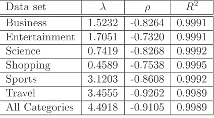
In order to fit a Weibull distribution to the averaged simulation data, following (V), we first adjusted the data as on the right-hand side of (15), in order to incorporate the first two correction terms in the Euler-Maclaurin summation formula. The value of k was chosen so that the error due to using the approximation ln(1 +x)≈xis small. We then calculated the right-hand side of (15) for each value of ifrom k to t, using the values ofF(i+ 1, t+ 1) and
F(k, t+ 1) from the simulation, and the values ofλand ρfrom Table 3. We then applied the exponential function to these values from (15) for each i, and used non-linear regression to fit the Weibull distribution in (11). We chose k= 10 after inspecting the values of λand ρ
Data set KM-Sim KM-Prod Sim-Prod
Business 0.0567 0.0561 0.0037
Entertainment 0.0189 0.0193 0.0030
Science 0.1082 0.1039 0.0046
Shopping 0.0756 0.0734 0.0052
Sports 0.0268 0.0246 0.0044
Travel 0.0741 0.0724 0.0055
[image:12.595.177.427.107.225.2]All Categories 0.0250 0.0219 0.0031
Table 4: TheD values for a 2-sample, 2-tailed Kolmogorov-Smirnov tests.
the R2 values indicate an almost perfect fit in all cases. It can be seen that the values of
λand ρ shown in Table 5 for the Weibull fit to the adjusted simulation data closely match those shown in Table 3 for the averaged simulation data. All the ρ values are between 0 and
−1, as expected.
Data set λ ρ R2
Business 1.5232 -0.8264 0.9991
Entertainment 1.7051 -0.7320 0.9991
Science 0.7419 -0.8268 0.9992
Shopping 0.4589 -0.7538 0.9995
Sports 3.1203 -0.8608 0.9992
Travel 3.4555 -0.9262 0.9989
All Categories 4.4918 -0.9105 0.9989
Table 5: Nonlinear least-squares regression to a Weibull for the adjusted simulation data with
k= 10.
6
Concluding Remarks
We have proposed a stochastic evolutionary urn model for survival analysis applications in the context of human dynamics. In our model, actors (represented by balls) remain in the system and survive until they die (i.e. are discarded) according to a specified mortality distribution, which may take a general form. A solution to the equations describing the model was obtained in the form of a product (3). We then obtained a continuous approximation to the solution (6) via the renewal equation from age-structured population dynamics. This provides a continuous analogue to our discrete stochastic urn-based model. Power-law mortality, which in the continuous case gives rise to the Weibull distribution (11), was used to model the survival of popular search engine queries. This could also be used to analyse the survival of Wikipedia editors [ZPL12], as well as other data sets relating to human behaviour.
[image:12.595.196.408.341.458.2]into the underlying processes and may also be useful for prediction purposes [HJS01]. In this context, extending the survival model, as in the Cox proportional hazard model [KK12], to allow the inclusion of features (known as risk factors) could give rise to more accurate predictions [LMS12].
Acknowledgements
We would like to thank Suneel Kingrani who collected the Google Trends data and computed the Kaplan-Meier estimates for the data set. We also thank the referees for their constructive comments, which helped us to improve the paper.
References
[AB02] R. Albert and A.-L. Barab´asi. Statistical mechanics of complex networks.Reviews of Modern Physics, 74:47–97, 2002.
[Apo99] T.M. Apostol. An elementary view of Euler’s summation formula. American Mathematical Monthly, 106:409–418, 1999.
[Bar05] A.-L. Barab´asi. The origin of bursts and heavy tails in human dynamics. Nature, 435:207–211, 2005.
[Bar07] A.-L. Barab´asi. The architecture of complexity: From network strucutre to hu-man dynamics. IEEE Control Systems Magazine, 27:33–42, 2007.
[BG03] C. Bracquemond and O. Gaudoin. A survey on discrete lifetime distributions.
International Journal of Reliability, Quality and Safety Engineering, 10:69–98, 2003.
[BSV07] S. B¨orner, S. Sanyal, and A. Vespignani. Network science. Annual Review of Information Science & Technology (ARIST), 41:537–607, 2007.
[CFL09] C. Castellano, S. Fortunato, and V. Loreto. Statistical physics of social dynamics.
Reviews of Modern Physics, 81:591–646, 2009.
[CGW+08] J. Candia, M.C. Gonz´alez, P. Wang, T. Schoenhar, G. Madey, and A.-L. Barab´asi. Uncovering individual and collective human dynamics from mobile phone records.
Journal of Physics A: Mathematical and Theoretical, 41:224015, 11pp, 2008.
[Cha94] B. Charlesworth. Evolution in age-structured populations. Cambridge Studies in Mathematical Biology: 13. Cambridge University Press, Cambridge, U.K., 2nd edition, 1994.
[CM06] A.G. Chessa and J.M.J. Murre. Modelling memory processes and internet re-sponse times: Weibull or power-law? Physica A, 366:539–551, 2006.
[EB14] M. Eagle and T. Barnes. Survival analysis on duration data in intelligent tutors. InProceedings of International Conference on Intelligent Tutoring Systems (ITS), pages 178–187, Honolulu, HI, 2014.
[FL00] T.R. Fleming and D.Y. Lin. Survival analysis in clinical trials: Past developments and future directions. Biometrics, 56:971–983, 2000.
[FLL07] T. Fenner, M. Levene, and G. Loizou. A model for collaboration networks giving rise to a power-law distribution with an exponential cutoff. Social Networks, 29:70–80, 2007.
[FLL12] T. Fenner, M. Levene, and G. Loizou. A discrete evolutionary model for chess players ratings. IEEE Transactions on Computational Intelligence and AI in Games, 4:84–93, 2012.
[FLL13] T. Fenner, M. Levene, and G. Loizou. A bi-logistic growth model for conference registration with an early bird deadline. Central European Journal of Physics, 11:904–909, 2013.
[FLL14] T. Fenner, M. Levene, and G. Loizou. A stochastic evolutionary model for survival dynamics. Physica A, 410:595–600, 2014.
[Gal08] S. Galam. Sociophysics: A review of Galam models. Journal of Modern Physics C, 19:409–440, 2008.
[GG01] L.A. Gavrilov and N.S. Gavrilova. The reliability theory of aging and longevity.
Journal of Theoretical Biology, 213:527–545, 2001.
[HJS01] R. Henderson, M. Jones, and J. Stare. Accuracy of point predictions in survival analysis. Statistics in Medicine, 20:3083–3096, 2001.
[HS98] P. Hedstr¨om and R. Swedberg. Social mechanisms: An introductory essay. In P. Hedstr¨om and R. Swedberg, editors, Social Mechanisms: An Analytical Ap-proach to Social Theory, pages 1–31. Cambridge University Press, Cambridge, U.K., 1998.
[KK12] D.G. Kleinbaum and M. Klein. Survival Analysis, A Self-Learning Text. Springer Science+Business Media, LLC, New York, NY, 3rd edition, 2012.
[KM58] E.L. Kaplan and P. Meier. Nonparametric estimation from incomplete observa-tions. Journal of the American Statistical Association, 53:457–481, 1958.
[LAE+
12] E. Lovecchio, P. Allegrini, E.Geneston, B.J. West, and P. Grigolini. From self-organized to extended criticality. Frontiers in Physiology, 3:Article 98, 9pp, 2012.
[Lam01] V. Lampret. The Euler-Maclaurin and Taylor formulas: Twin, elementary deriva-tions. Mathematics Magazine, 74:109–122, 2001.
[LB08] J. Li and F. Brauer. Continuous-time age-structured models in population dy-namics and epidemiology. In F. Brauer, P. van den Driessche, and J. Wu, editors,
Mathematical Epidemiology, Lecture Notes in Mathematics, Mathematical Bio-sciences Subseries, chapter 9, pages 205–227. Springer-Verlag, Berlin, 2008.
[LMS12] J.G. Lee, S. Moon, and K. Salamatian. Modeling and predicting the popularity of online contents with Cox proportional hazard regression model. Neurocomputing, 76:134–145, 2012.
[LS98] J. Laherr`ere and D. Sornette. Stretched exponential distributions in nature and economy: fat tails with characteristic scales. European Physical Journal B, 2:525– 539, 1998.
[MAAJ13] J. Mathiesen, L. Angheluta, P.T.H. Ahlgren, and M.H. Jensen. Excitable human dynamics driven by extrinsic events in massive communities. Proceedings of the National Academy of Sciences of the United States of America, 110:17259–17262, October 2013.
[Mot95] H. Motulsky. Intuitive Biostatistics. Oxford University Press, Oxford, 1995.
[MSR13] A. Mitnitski, X. Song, and K. Rockwood. Assessing biological aging: the origin of deficit accumulation. Biogerontology, 14:709–717, 2013.
[New05] M.E.J. Newman. Power laws, Pareto distributions and Zipf’s law. Contemporary Physics, 46:323–351, 2005.
[OK12] P.D.T. O’Connor and A. Kleyner. Practical Reliability Engineering. Wiley Series in Telecommunications. John Wiley & Sons, Chichester, 5th edition, 2012.
[PR91] M. Pilant and W. Rundell. Determining a coefficient in a first-order hyperbolic equation. SIAM Journal on Applied Mathematics, 51:494–506, 1991.
[PS10] R.K. Pan and S. Sinha. The statistical laws of popularity: universal properties of the box-office dynamics of motion pictures. New Journal of Physics, 12:115004 (23pp), 2010.
[Rin09] H. Rinne. The Weibull Distribution: A Handbook. CRC Press, Boca Raton, Fl., 2009.
[RNP+
10] J.T. Rich, J.G. Neely, R.C. Paniello, C.C.J. Voelker, B. Nussenbaum, and E.W. Wang. A practical guide to understanding Kaplan-Meier curves. Otolaryngology-Head and Neck Surgery, 143:331–336, 2010.
[Ros96] S.M. Ross. Stochastic Processes. John Wiley & Sons, New York, NY, 2nd edition, 1996.
[SBCG13] C.M. Schneider, V. Belik, T. Couronn´e, and M.C. Gonz´alez. Unravelling daily human mobility motifs.Journal of the Royal Society Interface, 10:20130246, 2013.
[Sch98] T.C. Schelling. Social mechanisms and social dynamics. In P. Hedstr¨om and R. Swedberg, editors,Social Mechanisms: An Analytical Approach to Social The-ory, pages 32–44. Cambridge University Press, Cambridge, U.K., 1998.
[Sim55] H.A. Simon. On a class of skew distribution functions. Biometrika, 42:425–440, 1955.
[TW02] A. Tsoularis and J. Wallace. Analysis of logistic growth models. Mathematical Biosciences, 179:21–55, 2002.
[VAFL10] P.O.S. Vaz De Melo, L. Akoglu, C. Faloutsos, and A.A.P. Loureiro. Surprising patterns for the call duration distribution of mobile phone users. InProceedings of European Conference on Machine Learning and Principles and Practice of Knowledge Discovery in Databases (ECML PKDD), pages 354–369, Barcelona, 2010.
[ZPL12] D. Zhang, K. Prior, and M. Levene. How long do wikipedia editors keep active? In