Model-Based Data Collection in Wireless Sensor Networks

Model-Based Data Collection in Wireless Sensor

Networks

Geeta Gupta*_{, Vinod Khandelwal}**_{, Vikas Gupta}***

*

Department of Computer Science, Indraprashtha College for Women(University of Delhi) 31, Sham Nath Marg, Delhi INDIA 110054

**

Research Scholar, MMICT & BM, MM University Mullana, Ambala, Haryana INDIA

***

VGAM Information Systems (P) Ltd., Faridabad

Abstract: Declarative queries are proving to be an attractive

paradigm for interacting with networks of wireless sensors. But sensors do not exhaustively represent the data in the real world. We have to map the raw sensor readings onto physical reality. In this paper, we enrich interactive sensor querying with statistical modelling techniques. We demonstrate that such models can help provide answers that are both more meaningful and more efficient to compute in both time and energy. Our approach works on several real world sensor-network data sets demonstrating that our model-based approach provides a high-fidelity representation of the real phenomena and leads to significant performance gains versus traditional data acquisition techniques.

Keywords- Wireless Sensor Network, Database Query, Tiny DB, TIDE

I. INTRODUCTION

Database technologies are starting to have a significant impact in the emerging area of wireless sensor networks. The area of sensornet querying represents an opportunity for database researchers to apply their expertise in this area of computer systems.

Declarative querying has proved powerful in allowing programmers to program for an entire network of sensor nodes rather than programming individual nodes. However, the statement that “the sensornet is a database” is misleading. Databases are treated as complete and authoritative sources of information. Database query engine answers a query based upon all the available data. Applying this approach to sensornets results in two problems:

1) Misrepresentations of data: In the sensornet environ-ment, it is not possible to gather all the data. The real world consists of a set of continuous phenomena in both time and space. Hence, the set of relevant data is in principle infinite. Sensing technologies acquire samples of physical phenomena at discrete points in time and space but the data acquired by the sensornet is unlikely to be a random sample of physical processes, for a number of reasons (non-uniform placement of sensors in space, faulty sensors, high packet loss rates, etc). So a straightforward interpretation of the

sensornet readings as a “database” may not be a reliable representation of the real world.

2) Inefficient approximate queries: Since a sensornet cannot acquire all possible data, any readings from a sensornet are “approximate”, in the sense that they only represent the true state of the world at the discrete in-stants and locations where samples were acquired. However, the leading approaches to query processing in sensornets [30, 21] follow a completist’s approach, acquiring as much data as possible from the environment at a given point in time, even when most of that data provides little benefit in approximate answer quality.

2.1. Our contribution

In this paper, we propose to compensate for both of these deficiencies by incorporating statistical models of real-world processes into a sensornet query processing architecture. The models can help provide more robust interpretations of sensor readings. For example, they can help identify sensors that are providing faulty data and can extrapolate the values of missing sensors or sensor readings at geographic locations where sensors are no longer operational. Furthermore, models provide a framework for optimizing the acquisition of sensor readings: sensors should be used to acquire data only when the model itself is not sufficiently rich to answer the query with acceptable confidence.

Underneath this architectural shift in sensornet querying, we define and address a key optimization problem: given a query and a model, choose a data acquisition plan for the sensornet to best refine the query answer. This optimization problem is complicated by two forms of dependencies - one in the statistical benefits of acquiring a reading and the other in the system costs associated with wireless sensor systems.

The second form of dependency hinges on the connectivity of the wireless sensor network. If the sensor node is not within radio range of the query source then one cannot acquire a reading from this node without forwarding the request/result pair through another node which is near. This presents not only a non-uniform cost model for acquiring readings but one with dependencies, due to multi-hop networking. The acquisition cost for near will be much lower if one has already chosen to acquire data from the node far by routing through near.

Here, we are building a prototype called TIDE that uses a specific model based on time-varying multivariate Gaussians. We explain how our model-based architecture and querying techniques are specifically applied in TIDE. We also present encouraging results on real-world sensornet trace data, demonstrating the advantages that models offer for queries over sensor networks.

II. OVERVIEW OF APPROACH

In this section, we provide an overview of our basic architecture and approach, as well as a summary of TIDE. Our architecture consists of a declarative query processing engine that uses a probabilistic model to answer questions about the current state of the sensor network. We describe a model as a probability density function p(X1,X2, . . . ,Xn), assigning a probability for each possible assignment to the attributes X1, X2 . . ,Xn where each Xi is an attribute of a particular sensor node(e.g., temperature on sensing node 7, voltage on sensing node 14). Typically, there is one such attribute per sensor type per sensing node. This model can also incorporate hidden variables (i.e., variables that are not directly observable),for example, whether a sensor is giving faulty values. Such models can be learned from historical data using standard algorithms.

Users query for information about the values of particular attributes or in certain regions of the network as they would in a traditional SQL database. Unlike database queries sensornet queries request real time information about the environment rather than information about a stored collection of data. The model is used to estimate sensor readings in the current time period; these estimates form the answer of the query. In the process of generating these estimates, the model may interrogate the sensor network for updated readings that will help to refine estimates for which its uncertainty is high. As time passes, the model may also update its estimates of sensor values, to reflect expected temporal changes in the data.

In TIDE, we use a specific model based on time-varying multivariate Gaussians. We describe this model below. However, our approach is general with respect to the model and more or less complex models can be used instead. The new models require no changes to the query processor and can reuse code that interfaces with and acquires particular readings from the sensor network. Figure 1 illustrates our basic architecture through an example.

Users submit SQL queries to the database. The queries include error tolerances and target confidence bounds that specify how much uncertainty the user is willing to tolerate. Such bounds will be intuitive to many scientific and

technical users, as they are the same as the confidence bounds used for reporting results in most scientific fields (c.f., the graph-representation shown in the upper right of Fig. 1). In this example the user is interested in estimates of the value of sensor readings for nodes numbered 1 through 8, within .1 degrees C of the actual temperature reading with 95% confidence. Based on the model, the system decides that the most efficient way to answer the query with the requested confidence is to read battery voltage from sensors 1 and 2 and temperature from sensor 4. Based on knowledge of the sensor network topology it generates an observation plan that acquires samples in this order and sends the plan into the network where the appropriate readings are collected. These readings are used to update the model, which can then be used to generate query answers with specified confidence intervals.

Figure 1: Architecture for model-based querying in sensor networks.

The model in this example chooses to observe the voltage at some nodes despite the fact that the user’s query was over temperature.

2.1. Confidence intervals and correlation models

Figure 2: Trace of voltage and temperature readings over a two day period from a single mote-based sensor.

Conversely, the user could have requested very wide confidence bounds, in which case the model may have been able to answer the query without acquiring any additional data from the network. In fact, in our experiments with TIDE on several real-world data sets, we see a number of cases where strong correlations between sensors during certain times of the day mean that even queries with relatively tight confidence bounds can be answered with a very small number of sensor observations. These tight confidences can be provided despite the fact that sensor readings have changed significantly. It is because known correlations between sensors make it possible to predict these changes: for example, in Figure 2, it is clear that the temperature on the two sensors is correlated given the time of day. During the daytime (e.g., readings 500-1000 and 2500-3000), sensor 20, which is placed near a window, is consistently hotter than sensor 5, which is in the center of our lab. A good model will be able to predict with high confidence that during daytime hours, sensor readings on sensor 20 are 1-2 degrees hotter than those at sensor 5 without actually observing sensor 20. This is in contrast to existing sensor network querying systems where sensors are continuously sampled and readings are always reported whenever small absolute changes happen.

Typically in probabilistic modeling, we pick a class of models, and use learning techniques to pick the best model in the class. The problem of selecting the right model class has been widely studied but can be difficult in some applications. In general, a probabilistic model is only as good at prediction as the data used to train it. Thus, it may be the case that the temperature between sensors 1 and 23 would not show the same relationship during a different season of the year, or in a different climate – in fact, one might expect that when the outside temperature is very cold, sensor 23 will read less than sensor 1 during the day, just as it does during the night time. Hence, for the models to perform accurate predictions they must be trained in the kind of environment where they will be used. That does not mean, however, that well-trained models cannot deal with changing relationships over time. The model we use in TIDE uses different correlation data depending on time of

day. For example, extending it to handle seasonal variations is a straight forward extension of the techniques we use for handling variations across hours of the day.

2.2.Networking model and observation plan format

Our initial implementation of TIDE focuses on static sensor networks, such as those deployed for building and habitat monitoring. For this reason, we assume that network topologies change relatively slowly. We capture network topology information when collecting data by including, for each sensor, a vector of link quality estimates for neighboring sensor nodes. We use this topology information when constructing query plans by assuming that nodes that were previously connected will still be there in future. When executing a plan if we observe that a particular link is not available (e.g., because one of the sensors has failed) then we update our topology model accordingly. We can continue to collect the new topology information as we query the network so that new links will also become available. This approach will be effective if the topology is relatively stable; highly dynamic topologies will need more sophisticated techniques.

In TIDE, observation plans consist of a list of sensor nodes to visit, and, at each of these nodes, a (possibly empty) list of attributes that need to be observed at that node. The possibility of visiting a node but observing nothing is included to allow plans to observe portions of the network that are separated by multiple radio hops. We require that plans begin and end at sensor id 0 (the root), which we assume to be the node that interfaces the query processor to the sensor network.

2.3. Cost model

During plan generation and optimization, we need to be able to compare the relative costs of executing different plans in the network. As energy is the primary concern in battery powered sensornets [15, 26], our goal is to pick plans of minimum energy cost. The primary contributors to energy cost are communication and data acquisition from sensors (CPU overheads beyond what is required when acquiring and sending data are small because there is no significant processing done on the nodes in our setting).

Sensor Energy Per

Sample (@3V), mJ Solar Radiation [29]

Barometric Pressure [16] Humidity and Temperature[28] Voltage

.525 0.003 0.5 0.00009

Table 1 : Power Requirements Summary of Crossbow MTS400 Sensorboard (From [20])

that both sender and receiver consume about .4 mJ of energy. Table 1 summarizes the energy costs of acquiring readings from various sensors available for motes. In this paper, we primarily focus on temperature readings. Assuming we are acquiring temperature readings (which cost .5 J per sample), we compute the cost of a plan that visits s nodes and acquires a readings to be (.4× 2)× s+.5× a if there are no lost packets. Note that this cost treats the entire network as a shared resource in which power needs to be conserved equivalently on each mote. More sophisticated cost models that take into account the relative importance of nodes close to the root could be used, but an exploration of such cost models is not needed to demonstrate the utility of our approach.

III. EXPERIMENTAL RESULTS

In this section, we measure the performance of TIDE on several real world data sets. Our goal is to demonstrate that TIDE provides the ability to efficiently execute approximate queries with user-specifiable confidences. 3.1. Data sets

Our results are based on running experiments over two real world data sets that we have collected during the past few months using TinyDB. The first data set, outside, is a one month trace of 83,000 readings from 11 sensors in a Botanical Garden. In this case, sensors were placed at 4 different altitudes in the tree, where they collected light, humidity, temperature, and voltage readings once every 5 minutes. We split this data set into non-overlapping training and test data sets (with 2/3 used for training) and build the model on the training data. The second data set, inside, is a trace of readings from 54 sensors in the lab. These sensors collected light, humidity, temperature and voltage readings, as well as network connectivity information that makes it possible to reconstruct the network topology. Currently, the data consists of 8 days of readings; we use the first 6 days for training, and the last 2 for generating test traces.

3.2.Query workload

We report results for the two sets of query workloads- Value Queries: The main type of queries that we anticipate users would run on a such a system are queries asking to report the sensor readings at all the sensors, within a specified error bound € with a specified confidence ∂, indicating that no more than a fraction 1−∂of the readings should deviate from their true value by €. As an example, a typical query may ask for temperatures at all the sensors within 0.5 degrees with 95% confidence.

Predicate Queries: The another set of queries that we use are selection queries over the sensor readings where the user asks for all sensors that satisfy a certain predicate and once again specifies a desired confidence .

We also looked at average queries asking for averages over the sensor readings.

Comparison systems

We compare the effectiveness of TIDE against two simple strategies for answering such queries :

TinyDB-style Querying: In this model, the query is disseminated into the sensor network using an overlay tree structure [22], and at each mote, the sensor reading is observed. The results are reported back to the base station

using the same tree, and are combined along the way back to minimize communication cost.

Approximate-Caching: The base-station maintains a view of the sensor readings at all motes that is guaranteed to be within a certain interval of the actual sensor readings by requiring the motes to report a sensor reading to the base station if the value of the sensor falls outside this interval. Note that, though this model saves communication cost by not reporting readings if they do not change much, it does not save acquisition costs as the motes are required to observe the sensor values at every time step.

3.4.Methodology

TIDE is used to build a model of the training data. This model includes a transition model for each hour of the day. We generate traces from the test data by taking one reading randomly for each hour and we issue one query against this model per hour. The model computes the a priori probabilities for each predicate (or € bound) being satisfied, and chooses one or more additional sensor readings to observe if the confidence bounds are not met. After executing the generated observation plan over the network (at some cost), TIDE updates the model with the observed values from the test data and compares predicted values for non-observed readings to the test data from that hour. To measure the accuracy of our prediction with value queries, we compute the average number of mistakes (per hour) that TIDE made, i.e., how many of the reported values are further away from the actual values than the specified error bound. To measure the accuracy for predicate queries we compute the number of predicates whose truth value was incorrectly approximated.

For TinyDB, all queries are answered “correctly” (as we are not modeling loss). Similarly, for approximate caching, a value from the test data is reported when it deviates by more than € from the last reported value from that sensor, and as such, this approach does not make mistakes either. We compute a cost for each observation plan as described above; this includes both the attribute acquisition cost and the communications cost. For most of our experiments, we measure the accuracy of our model at predicting temperature.

3.5.Outside dataset: Value-based queries

“mistakes”, although the average observation error in approximate caching is close to TIDE (for example, in this experiment, with epsilon=.5, approximate caching has a root-mean squared error of .46, whereas TIDE this error is .12; in other cases the relative performance is reversed).

Figure 3 : Fig. showing the relative costs of TIDE versus TinyDB

Figure 4: Fig. showing the number of sensors observed over time for varying epsilons.

Fig. 4 shows the percentage of sensors that TIDE observes by hour with varying epsilon for the same set of outside experiments. As epsilon gets small (less than .1 degrees) it is necessary to observe all nodes on every query as the variance between nodes is high enough that it cannot infer the value of one sensor from other sensor’s readings with such accuracy. On the other hand, for epsilons 1 or larger, very few observations are needed, as the changes in one sensor closely predict the values of other sensors. For intermediate epsilons, more observations are needed, especially during times when sensor readings change dramatically. The spikes in this case correspond to morning and evening, when temperature changes relatively quickly as the sun comes up or goes down (hour 0 in this case is midnight).

3.6. Outside Dataset: Cost vs. Confidence

For our next set of experiments, we again look at the Outside data set, this time comparing the cost of plan execution with confidence intervals ranging from 99% to 80%, with epsilon again varying between 0.1 and 1.0. The results are shown in Figure 5(a) and (b). Figure 5(a) shows that decreasing confidence intervals substantially reduces the energy per query, as does decreasing epsilon. Note that for a confidence of 95% with errors of just .5 degrees C we can reduce expected per query energy costs from 5.4 J to less than 150 mJ – a factor of 40 reduction. Figure 5(b) shows that we meet or exceed our confidence interval in almost all cases (except 99% confidence). It is not

surprising that we occasionally fail to satisfy these bounds by a small amount, as variances in our training data are somewhat different than variances in our test data.

Figure 5: Energy per query (a) and percentage of errors (b) versus confidence interval size and epsilon.

We also ran experiments comparing (1) the performance of the greedy algorithm vs. the optimal algorithm, and (2) the performance of the dynamic (Kalman Filter) model that we use vs. a static model that does not incorporate observations made in the previous time steps into the model. As expected, the greedy algorithm performs slightly worse that the optimal algorithm, whereas using dynamic models results in less observations than using static models.

3.7.Outside Dataset: Range queries

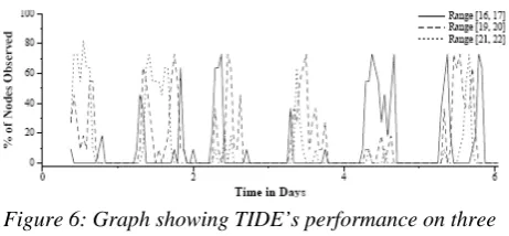
We ran a number of experiments with range queries (also over the outside data set). Figure 6 summarizes the average number of observations required for a 95% confidence with three different range queries (temperature in [17,18], temperature in [19,20], and temperature in [20,21]). In all three cases, the actual error rates were all at or below 5% (ranging from 1.5- 5%). Notice that different range queries require observations at different times – for example, during the set of readings just before hour 50, the three queries make observations during three disjoint time periods: early in the morning and late at night, the model must make lots of observations to determine whether the temperature is in the range 16-17, whereas during mid-day, it is continually making observations for the range 20-21 but never for other ranges.

Figure 6: Graph showing TIDE’s performance on three different range queries, for the garden data set with

confidence set to 95%.

3.8.Inside dataset

set of experiments for this dataset, but defer a more detailed study to future work.

Figure 7(a) shows the cost incurred in answering a value query on this dataset, as the confidence bound is varied. For comparative purposes, we also plot the cost of answering the query using TinyDB. Once again, we see that as the required confidence in answer drops, TIDE is able to answer the query more efficiently, and is significantly more cost-efficient than TinyDB for larger error bounds. Figure 7(b) shows that TIDE was able to achieve the specified confidence bounds in almost all the cases.

Figure 7: Energy per query (a) and percentage of errors (b) versus confidence interval size and epsilon for the Inside

Data.

IV. EXTENSIONS AND FUTURE DIRECTIONS

In this paper, we focused on the core architecture for unifying probabilistic models with declarative queries. In this section we outline several possible extensions.

Conditional plans: In our current prototype, once an observation plan has been submitted to the sensor network, it is executed to completion. A simple alternative would be to generate plans that include early stopping conditions; a more sophisticated approach would be to generate conditional plans that explore different parts of the network depending on the values of observed attributes. We have begun exploring such conditional plans in a related project [8].

More complex models: In particular, we are interested in building models that can detect faulty sensors, both to answer fault detection queries, and to give correct answers to general queries in the presence of faults. This is an active research topic in the machine learning community (e.g., [18]), and we expect that these techniques can be extended to our domain.

Outliers: Our current approach does not work well for outlier detection. To a first approximation, the only way to detect outliers is to continuously sample sensors, as outliers are fundamentally uncorrelated events. Thus, any outlier detection scheme is likely to have a high sensing cost, but we expect that our probabilistic techniques can still be used to avoid excessive communication during times of normal operation, as with the fault detection case.

Support for dynamic networks: Our current approach of re-evaluating plans when the network topology changes

will not work well in highly dynamic networks. As a part of our instrumentation of our lab space, we are beginning a systematic study of how network topologies change over time and as new sensors are added or existing sensors move. We plan to use this information to extend our exploration plans with simple topology change recovery strategies that can be used to find alternate routes through the network.

Continuous queries: Our current approach re-executes an exploration plan that begins at the network root on every query. For continuous queries that repeatedly request data about the same sensors, it may be possible to install code in the network that causes devices to periodically push readings during times of high change (e.g., every morning at 8 am).

V. RELATED WORK

There has been substantial work on approximate query processing in the database community, often using model-like synopses for query answering much as we rely on probabilistic models. For example, the AQUA project [12, 10, 11] proposes a number of sampling-based synopses that can provide approximate answers to a variety of queries using a fraction of the total data in a database. As with TIDE, such answers typically include tight bounds on the correctness of answers. AQUA, however, is designed to work in an environment where it is possible to generate an independent random sample of data (something that is quite tricky to do in sensor networks, as losses are correlated and communicating random samples may require the participation of a large part of the network). AQUA also does not exploit correlations which mean that it lacks the predictive power of representations based on probabilistic models. [7, 9] propose exploiting data correlations through use of graphical model techniques for approximate query processing, but neither provide any guarantees in the answers returned. Recently, Considine etal. have shown that sketch based approximation techniques can be applied in sensor networks [17].

Work on approximate caching by Olston et al., is also related

[25, 24], in the sense that it provides a bounded approximation

of the values of a number of cached objects (sensors, in our case) at some server (the root of the sensor network). The basic idea is that the server stores cached values along with absolute bounds for the deviation of those values; when objects notice that their values have gone outside the bounds known to be stored at the server, they send an update of our value. Unlike our approach, this work requires the cached objects to continuously monitor their values, which makes the energy overhead of this approach considerable. It does, however, enable queries that detect outliers, something TIDE currently cannot do.

queries that estimate the most likely value of a cached object as well as an confidence on that uncertainty. As with other approximation work, the notion of correlated values is not exploited, and the requirement that readings be continuously monitored introduces a high sampling overhead.

Information Driven Sensor Querying (IDSQ) from Chu et al. [4] uses probabilistic models for estimation of target position in a tracking application. In IDSQ, sensors are tasked in order according to maximally reduce the positional uncertainty of a target, as measured, for example, by the reduction in the principal components of a 2D Gaussian.

Our prior work presented the notion of acquisitional query processing(ACQP) [21] – that is, query processing in environments like sensor networks where it is necessary to be sensitive to the costs of acquiring data. The main goal of an ACQP system is to avoid unnecessary data acquisition. The techniques we present are very much in that spirit, though the original work did not attempt to use probabilistic techniques to avoid acquisition, and thus cannot directly exploit correlations or provide confidence bounds.

TIDE is also inspired by prior work on Online Aggregation [14] and other aspects of the CONTROL project [13]. The basic idea in CONTROL is to provide an interface that allows users to see partially complete answers with confidence bounds for long running aggregate queries. CONTROL did not attempt to capture correlations between the different attributes, such that observing one attribute had no effect on the systems confidence on any of the other predicates.

The probabilistic querying techniques described here are built on standard results in machine learning and statistics (e.g., [27, 23, 5]). The optimization problem we address is a generalization of the value of information problem [27]. This paper, however, proposes and evaluates the first general architecture that combines model-based approximate query answering with optimizing the data gathered in a sensornet.

VI. CONCLUSIONS

In this paper, we proposed a novel architecture for integrating a database system with a correlation-aware probabilistic model. Rather than directly querying the sensor network, we build a model from stored and current readings, and answer SQL queries by consulting the model. In a sensor network, this provides a number of advantages including shielding the user from faulty sensors and reducing the number of expensive sensor readings and radio transmissions that the network must perform. Beyond the encouraging, order-of-magnitude reductions in sampling and communication cost offered by TIDE, we see our general architecture as the proper platform for answering queries and interpreting data from real world environments like sensornets, as conventional database technology is poorly equipped to deal with lossiness, noise, and non-uniformity inherent in such environments.

REFERENCES

[1] IPSN 2004 Call for Papers. http://ipsn04.cs.uiuc.edu/ call_for_papers.html.

[2] SenSys2004 Call for Papers. http://www.cis.ohio-state.edu/sensys04/.

[3] R. Cheng, S. Prabhakar and D. V. Kalashnikov. Evaluating probabilistic queries over imprecise data. In SIGMOD 2003.

[4] M. Chu, F. Zhao and H. Haussecker. Scalable information-driven sensor querying and routing for ad hoc heterogeneous sensor-networks: In Journal of High Performance Computing Applications

2002.

[5] R. Cowell, S. Lauritzen, P. Dawid, and D. Spiegelhalter.

Probabilistic Networks and Expert Systems. Spinger New York

1999.

[6] Crossbow, Inc. Wireless sensor networks. http://www.xbow.com/Products/Wireless_Sensor_Networks.htm.

[7] R. Rastogi , A. Deshpande and M. Garofalakis. Independence is Good: Dependency-Based Histogram Synopses for High-Dimensional Data. In SIGMOD, May 2001.

[8] A. Desphande, W. Hong, C. Guestrin, and S. Madden. Exploiting correlated attributes in acquisitional query processing, Technical report, Intel-Research Berkeley, 2004.

[9] B. Taskar, L. Getoor, and D. Koller. Selectivity estimation using probabilistic models. In SIGMOD, May 2001.

[10] P. B. Gibbons. Distinct sampling for highly-accurate answers to distinct values queries and event reports. In Proc. of VLDB, Sept 2001.

[11] M. Garofalakis and P. B. Gibbons. Approximate query processing: Taming the terabytes (tutorial), September 2001.

[12] Y. Matias and P. B. Gibbons. New sampling based summary statistics for improving approximate query answers. In SIGMOD

1998.

[13] A. Chou, J. M. Hellerstein, R. Avnur, C. Hidber, C. Olston, V. Raman, T. Roth, and P. J. Haas. Interactive data analysis with CONTROL, IEEE Computer 32(8) August 1999.

[14] J. M. Hellerstein, P. J. Haas, and H. Wang. Online aggregation. In

SIGMOD, pages 171–182, Tucson, AZ, May 1997.

[15] C. Intanagonwiwat, R. Govindan, and D. Estrin. Directed diffusion: A scalable and robust communication paradigm for sensor networks. In MobiCOM Boston MA, August 2000.

[16] Intersema. Ms5534a barometer module. Technical report, October 2002 http://www.intersema.com/pro/module/file/da5534.pdf. [17] G. Kollios, J. Considine, F. Li, and J. Byers. Approximate

aggregation techniques for sensor databases. In ICDE 2004. [18] U. Lerner, B. Moses, M. Scott, S. McIlraith, and D. Koller.

Monitoring a complex physical system using a hybrid dynamic bayes net. In UAI, 2002.

[19] S. Lin and B. Kernighan. An effective heuristic algorithm for the tsp.

Operations Research, 21:498–516, 1971.

[20] S. Madden. The design and evaluation of a query processing architecture for sensor networks. Master’s thesis, UC Berkeley, 2003. [21] S. Madden, M. J. Franklin, J. M. Hellerstein, and W. Hong. The

design of an acquisitional query processor for sensor networks. In

ACM SIGMOD, 2003.

[22] S. Madden, W. Hong, J. M. Hellerstein, and M. Franklin. TinyDB web page. http://telegraph.cs.berkeley.edu/tinydb.

[23] T. Mitchell. Machine Learning. McGraw Hill, 1997.

[24] C. Olston and J.Widom. Best effort cache sychronization with source cooperation. SIGMOD, 2002.

[25] C. Olston, B. T. Loo, and J. Widom. Adaptive precision setting for cached approximate values. In ACM SIGMOD, May 2001.

[26] G. Pottie andW. Kaiser. Wireless integrated network sensors.

Communications of the ACM, 43(5):51 – 58, May 2000.

[27] S. Russell and P. Norvig. Artificial Intelligence: A Modern Approach. Prentice Hall, 1994.

[28] Sensirion. Sht11/15 relative humidity sensor. Technical report, June 2002.

http://www.sensirion.com/en/pdf/Datasheet_SHT1x_SHT7x_0206.p df.

[29] TAOS, Inc. Tsl2550 ambient light sensor. Technical report, September 2002. http://www.taosinc.com/pdf/tsl2550-E39.pdf. [30] Y. Yao and J. Gehrke. Query processing in sensor networks. In