!
"
# #
"$ % %#
&
''' (
Stroke Risk Prediction through Non-linear Support Vector Classification Models
Sabibullah Mohamed Hanifa
*
Asst. Prof., Dept. of MCA, JJ College of Engg. & Technology,Trichirappalli, Tamilnadu ,India [email protected]
Kasmir Raja S.V
Dean (Research), SRM University, Kattankulathur, Chennai,Tamilnadu, India, [email protected]
Abstract: The aim of this study is to find the possible risk of Cerebro Vascular Accident (CVA) or Stroke by subjecting the risk factors to Support Vector Machines (SVM).The prediction of the attack of the disease is highly dependent on the quantification of risks contributed by each factor. Therefore an assessment of relative intensity of risk contributed by the factors is imperative for early prediction and preventable measures. The classification accuracies are achieved through the efficient kernel functions of Radial Basis Function (RBF=98%) and Polynomial (Poly=92%) and finally these results are compared with benchmarking evaluation methods like classification accuracy, sensitivity, specificity and confusion matrix. The proposed stroke risk prediction models are obtained with satisfactory accuracy and it would be promising models in the classification of stroke risk prediction process.
Keywords: Support Vector Machines, Cerebrovascular Accident, Stroke Risk factors, Classification, Kernel Functions.
I. INTRODUCTION
Stroke is defined by the National Institute of Neurological Disorders and Stroke (NINDS), USA as a sudden loss of brain function resulting from an interference with blood supply to the brain. The brain receives about 25% of the body's oxygen, but it cannot store it. Brain cells require a constant supply of oxygen to stay healthy and function properly. From 1995-2005 the stroke death rate fell approximately 30%. However it is reported that 80% of strokes are preventable. Medical diagnosis systems and disease prediction tools using different machine learning approaches have shown great potential. In the last two decades, the uses of machine learning tools have become widely accepted in medical applications to support patients in effective management of disease and also in preventive measurements. The aim and use of Support Vector Machine (SVM) is to devise a computationally efficient way of learning in classification. Hence, relative risk on stroke and risk factors reduction is an important step in preventing stroke and also this study would assist the primary and secondary treatment interventions. The proposed stroke risk prediction of mathematical models based on non-linear Support Vector Classification (SVC) would be a promising tool in the classification of stroke risk prediction process.
II. RELATED WORKS
Application of various machine learning approaches such as Decision Trees (DTs), Artificial Neural Networks (ANN), Bayesian Networks (BN), and Support Vector Machines (SVMs) have been actively tried to meeting clinical support requirements. In SVM technique, structural risk minimization is used whereas in ANN technique empirical risk minimization is used. By the strength of the statistical learning theory [26], SVMs are not only popular
in the machine learning and mathematics community also. Research efforts have reported with increasing confirmation that the SVM has greater accurate diagnosis ability. Different aspects of research in stroke have been studied by various researchers by their different approaches [2], [3], [7],[10], [15], [16], [17], [18], [20], [21], [23], and [24]. The interpreted results in these existing approaches having the different properties and also merits and demerits in its accuracy produced. The use of classifier systems in medical diagnosis is increasing gradually [12]. SVM has been used as a classification tool with a great deal of success in a variety of areas ranging from Cardiovascular disease prediction [22], a DSS based on SVM for diagnosis of the heart valve diseases [8], an application to hypertension diagnosis [4], classification of diabetes disease [12], prediction model building in breast cancer diagnosis [5]. Current treatments for patients with established stroke are relatively ineffective and risk factor interventions are real hope in reducing morbidity and mortality in populations [9] and [1].
III. MATERIALS AND METHODS
A. Proposed Modeling
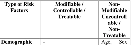
[image:1.612.321.548.660.738.2]Risk factors for stroke are well documented. Prediction [13] about the course of risk factors of the stroke is a key component of healthcare decision-making process.
Table 1 Classification of stroke risk factors
Type of Risk Factors
Modifiable / Controllable /
Treatable
Non-Modifiable Uncontroll
able / Non-Treatable
and Race
Lifestyle Cigarette Smoking,
Alcohol use and
Obesity / Excessive weight.
-
Medical / Clinical
Hypertension, Diabetes
Mellitus, Atrial
fibrillation, Lipid
profiles: Total
cholesterol, HDL, LDL and Triglycerides.
Previous history of stroke or TIA, Family History of stroke and heart disease.
Functional Physical Activity / Exercise
-
Major risk factors for stroke might be considered as main targets for primary and secondary prevention of stroke. More individual risk factors may help to improve the individual risk assessment[19]. In this line of research, we proposed the SVC stroke risk prediction models from its risk factors, is experimented through the effective kernel functions of RBF and Polynomial kernels. Its parameters are described in Table 2. Many risk factors can be changed or managed, while others cannot be changed. There are two clusters of stroke risk factors which are explained in Table 1.
B. Support vector machines methodology:
Support Vector Machines (SVM) recognized in the theory of Statistical Learning Theory (SLT) and a newly proposed method of Machine Learning has some outstanding advantages and it can be used for Support Vector Classification (SVC) and Support Vector Regression (SVR). It is suitable for both linear and nonlinear data processing; it has special generalization ability, especially for problems of small size. SVMs make predictions by automated learning from existing knowledge [26]. This type of learning requires training data where the answer is known so that rules or other functions that fit the data can be generated. The aim of SVM is to devise a computationally efficient way of learning in classification. It can separate the classes with a particular hyper plane which maximizes a quantity called ‘margin’. The margin is the distance from a hyper plane separating the classes to the nearest point in the dataset. In binary classification, we are given a set of input vectors {xi}, x
∈
ℜ
ntogether with the corresponding class labels {yi} where yi
∈
{1,-1}. The goal is to infer an information f(y) based on the training set. This can be done by choosing a learning model f(.) which is controlled by some unknown parameters x, and “learning” these parameters from the given training set. SVMs [6],are one of the most popular methods and make predictions based on the classification decision function; i.e., Structural RiskMinimization (SRM) principle,
+
=
= sv
n
1 i
i i
i
y
k(x
,
y)
b
sgn
)
(
y
α
f
(1)where yi are the labels,
α
iare the Lagrange multipliers (it isa systematic way of generating the necessary conditions for a stationary point), xi is the support vectors previously identified through the training process, and y is the test data
vector. Here,
α
i≥0 ,i=1,2,...,n (where ‘n’ is the number of support vectors) are non-negative Lagrange Multipliers thatsatisfy
0
1
=
= ni i i
y
α
. In equation (1), kernel function andweight vector ‘x’ are the parameters of the model. The success of SVM is attributed to the margin maximization theory [26].k (xi, y) for i=1, 2… n represents a symmetric positive definite kernel functions that defines an inner product in the feature space. In a typical classification task, only a small subset of the Lagrange multipliers
α
i usuallytends to be >0. The respective training vectors having non-zero which are closest to the optimal hyper plane (
α
i) arecalled support vectors or latency vectors. These support vectors will be formed into a model by the SVM. For training, SVMs use a quadratic optimization problem [25]. The construction of a hyper plane wTx+b=0 (w is the vector of hyper plane co-efficient [Input vectors], b is a bias term and x is an adaptive weight vector).
C. Setting support vector classification model parameters through its kernel function
SVM can present mathematical models with better prediction ability. Support Vector Classification (SVC) has been used as a mathematical modeling in this work for both SVMRBF and SVMPoly machines. The performance of SVC modeling is dependent on the combination of several factors, including the parameter C, the kernel type and its corresponding parameters. The kernel functions Gaussian RBF and Polynomial have been selected in this investigation to generate the stroke risk prediction through the task of SVC. No specific kernel functions have the best generalization performance for all kind of problem domains. The decision on selecting appropriate values of d is basically by trial and error. SVM maps the training samples from the input space into a higher dimensional feature space via a mapping function
φ
. The kernel function k (xi, xj) defines aninner product as k (xi, xj) =
φ
(xi).φ
( xj ). Usually the inner products are replaced by kernel function in the dual Lagrange. The following different kernel functions are used in our SVC stroke risk prediction modeling.1. Polynomial kernel: K(x,x’) = (x.x’+1)d ;
where d is the degree of kernel and positive integer number.
2. Gaussian (RBF) kernel : K(x,x’) = exp(-||x-xi’||2 /
σ
2 ); whereσ
is a positive real number.IV. EXPERIMENTAL RESULTS
[image:2.612.54.287.49.229.2]Table 2 SVM kernels and their corresponding kernel specific parameters
Hypersurafce kernel type
Kernel specific parameters
Parameters Value
Polynomial Even degree (d)
2
Gaussian (RBF)
Kernel width (
γ
)0.01
Performance analysis data have been classified by SVC and are listed in Table 6 by using Gaussian RBF and Polynomial kernels. The rate of correctness of prediction by RBF is 98% and by Polynomial is 92%. It proves that the application of SVC models can be used for the processing of stroke related risk factors data. Also, it implies that our models have good generalization ability. In this research work, we used the SVMLight software for implementation.
A. RBF modeling
Using the RBF kernel function with capacity parameter C= 100, the following criterion for the stroke risk prediction has been obtained through classification decision function.
)
(
∈
=
sv i
i i
y
x
f
α
exp (-||x-xi’||2 /σ
2) -0.3113364 (2) where b= -0.3113364,
σ
=0.01,α
i (listed in Table 3) arecorresponding to the Lagrange multipliers of support vectors. yi =1 corresponds to the samples of class 1; while yi
[image:3.612.98.515.291.566.2]= -1 corresponds to the samples of class 2. x is a vector (pattern of sample) with unknown activity to be discriminated; xi is one of the support vectors.
f
(
x
)
≥
0
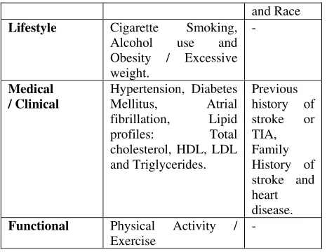
corresponds to class 1. In this stroke risk prediction models using the RBF kernel function with the aforesaid parameters are used for mathematical model building (see equation 2).Table 3: The sample number of support vectors and their corresponding coefficients for the kernel of Gaussian RBF kernel Sample
No.
α
i
Sample
No.
α
i
Sample
No.
α
i
Sample
No.
α
i
1 0.59325 18 0.59325 37 -0.59325 56 -0.59325
2 -0.59325 19 0.59325 38 -0.59325 57 0.59325
3 0.59325 20 -0.46380 39 -0.59325 58 0.59325
4 0.59325 22 -0.59325 41 0.59325 60 -0.59325
5 0.59325 24 0.59325 43 -0.59325 62 0.59325
6 -0.59325 25 0.59325 45 0.59325 63 -0.59325
7 -0.59325 26 -0.47678 46 -0.59325 65 0.59325
8 -0.59325 28 0.59325 48 0.59325 67 -0.59325
11 0.59325 29 -0.59325 49 0.59325 68 -0.17322
12 -0.50880 30 -0.59325 50 -0.59325 69 -0.59325
13 -0.59325 32 0.59325 51 0.59325 71 0.59325
15 0.59325 33 -0.59325 52 -0.59325 72 -0.12727
16 -0.59325 35 0.59325 54 0.59325 73 -0.59325
17 0.17323 36 0.59325 55 0.34573 75 0.00891
B. Polynomial modeling
With the evident of experimental results, the polynomial kernel function (even degree d=2) with c=100 has been used for modeling by SVC. The mathematical model (see equation 3) obtained can be expressed as follows.
P75 =
β
i[(
x
i.x
)
+
1
]
2 + (-2.8246306) (3)where
β
i (listed in Table 4) is the Lagrange coefficients corresponding to support vectors. x is a vector with unknown activity. xi is one of the support vectors. All support vectors obtained are presented in Table 4. The results of stroke risk prediction of the mathematical model built by SVC are more reliable. Hence SVM has beenconsidered as a new powerful tool for the prediction of stroke risk.
C. Real data set of stroke
1. Hypertension 2. Diabetes Mellitus 3. Obesity 4. Cigarette Smoking 5. Heart Disease 6. Prior Stroke /TIA 7. High Cholesterol and 8. Physical Activity/ Exercise. These eight attributes (variables) for each patient’s data are pre-processed by means of positive real values; finally this forms a training set and test set.
The details are;
Total no. of Input attributes : 08
Total no. of Output attribute : 01 (Training set) Total no. of Class Labels : 02 (Class 1[+1] and Class 2 [-1])
Total no. of Training samples : 75 Total no. of Testing samples : 25
[image:4.612.103.512.152.634.2]Regularization Parameter value (C) :100 (for both RBF and Polynomial kernels)
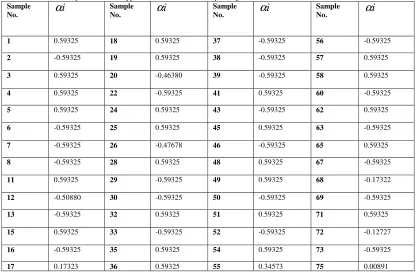
Table 4: The sample no. of support vectors and their corresponding coefficients for the kernel of polynomial
Sample
No.
β
iSample
No.
β
iSample
No.
β
iSample
No.
β
i1 0.13253 20 -0.13253 38 -0.13253 57 0.13253
2 -0.13253 21 0.13253 39 -0.13253 58 0.13253
4 0.13253 22 -0.13253 41 -0.13253 59 -0.13253
5 0.13253 24 0.13253 42 -0.13253 60 -0.13253
6 -0.13253 25 0.13253 43 -0.13253 62 0.13253
7 -0.13253 26 -0.13253 45 0.13253 63 -0.13253
8 -0.13253 27 0.13253 46 -0.13253 65 0.13253
10 0.13253 28 0.13253 48 0.13253 66 0.13253
11 0.13253 29 -0.13253 49 0.13253 67 -0.13253
12 -0.13253 30 -0.13253 50 -0.13253 68 -0.13253
13 -0.13253 32 0.13253 51 0.13253 69 -0.13253
15 0.13253 33 -0.13253 52 -0.13253 71 0.13253
16 -0.13253 35 0.13253 54 0.13253 72 -0.13253
18 0.13253 36 0.13253 55 0.13253 73 -0.13253
19 0.13253 37 -0.13253 56 -0.13253 75 0.13253
Table 5: Class labeling of stroke patient’s data set
Sample No. Class Sample No.
Class Sample No.
Class Sample No.
Class
1 C2 26 C1 51 C2 76 C1
2 C1 27 C2 52 C1 77 C2
3 C1 28 C1 53 C1 78 C1
4 C1 29 C1 54 C2 79 C1
5 C2 30 C1 55 C2 80 C1
6 C1 31 C2 56 C1 81 C2
7 C2 32 C2 57 C1 82 C1
8 C2 33 C2 58 C2 83 C1
9 C1 34 C1 59 C1 84 C2
10 C1 35 C1 60 C1 85 C2
11 C1 36 C1 61 C1 86 C1
12 C2 37 C2 62 C2 87 C1
13 C2 38 C2 63 C2 88 C2
14 C1 39 C1 64 C2 89 C1
15 C1 40 C1 65 C1 90 C1
16 C2 41 C2 66 C1 91 C1
17 C1 42 C1 67 C2 92 C2
18 C1 43 C1 68 C2 93 C2
19 C1 44 C1 69 C1 94 C2
20 C2 45 C2 70 C1 95 C1
21 C1 46 C1 71 C2 96 C1
22 C1 47 C2 72 C1 97 C2
23 C2 48 C1 73 C1 98 C2
24 C2 49 C1 74 C1 99 C1
25 C1 50 C1 75 C2 100 C1
*“Class 1 (C1)” denotes the samples of stroke disease patients and “Class 2 (C2)” denotes those of prone risk patients.
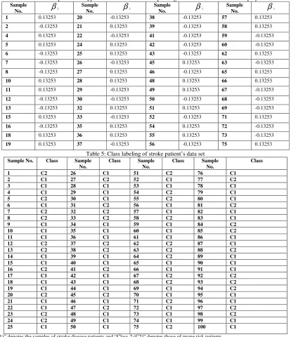
D. Performance metrics
We have used four methods for performance evaluation of stroke risk prediction. These are classification accuracy, two epidemiological indices (i.e., sensitivity analysis, specificity analysis) and confusion matrix. Table 6 shows the classification accuracy predicted by our SVC models
through test data set. Computing formula for Sensitivity and Specificity analysis is as below.
Sensitivity (True positive achieved) = TPTPFN
%
+
Specificity (True negatives achieved) = FPTNTN
%
+
[image:4.612.99.513.156.636.2]Statistical Measures SVM
RBF
SVM
Poly
Total Classification Acc (%) in test set
98 % 92 %
Sensitivity 93 % 100%
Specificity 100 % 80%
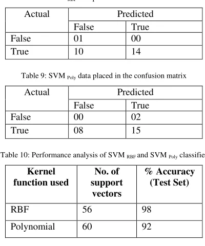
E. Confusion matrix
A confusion matrix is a method of finding an error measure and it contains information about actual and predicted classifications done by a classification system. Performance of a system is commonly evaluated using the data in the matrix. Table 7 shows the confusion matrix for a two class classifier. The entries in the confusion matrix are;
1. a is the number of correct predictions that an instance is negative,
2. b is the number of incorrect predictions that an instance is positive,
3. c is the number of incorrect predictions that an instance is negative and
[image:5.612.69.277.51.153.2]4. d is the number of correct predictions that an instance is positive.
Table 7: Representation of Confusion Matrix
Actual Predicted
False True
False FNc FPb
True TNa TPd
[image:5.612.323.509.112.201.2]where TP, TN, FP and FN denotes true positives, true negatives, false positives and false negatives respectively.
Table 8: SVM RBF data placed in the confusion matrix
Actual Predicted
False True
False 01 00
True 10 14
Table 9: SVM Poly data placed in the confusion matrix
Actual Predicted
False True
False 00 02
True 08 15
Table 10: Performance analysis of SVM RBF and SVM Poly classifier
Kernel function used
No. of support
vectors
% Accuracy (Test Set)
RBF 56 98
Polynomial 60 92
F. Evaluation of error prediction of mathematical models Results of the prediction of mathematical models are validated and compared with accuracy metrics. The evaluation metrics are Mean Absolute Error (MAE), Upside Mean Absolute Error (UMAE) and Downside Mean
Absolute Error (DMAE) is computed with the respective formulas (see equation 4 to 6) and the values are tabulated in Table 11. These metrics are used to evaluate the prediction performance. Mean Absolute Error is used to find a measure of the discrepancy between the actual and predicted values.
MAE = 1/m *
=
−
mi
pi
xi
1|
|
(4)UMAE = 1/m *
≥ =
−
mpi xi i
pi
xi
, 1)
(
(5)DMAE = 1/m *
=
−
mpi xi i
xi
pi
, 1)
(
(6) [image:5.612.336.540.255.548.2](where ‘xi’ and ‘pi’ are the actual and predicted values. ‘m’ is the number of testing data).
Table 11: Error of prediction of mathematical models obtained by SVMRBF
and SVMPoly
Method of classifica tion
MAE UMAE DMAE
SVM RBF 0.275215 -0.085039 0.085039
SVM Poly 0.402814 -0.187087 0.187087
Table 12: Stroke data set statistical analysis
Name of the Attribute
Mean Value Standard Deviation Hypertension 0.6116 0.1131
Diabetes 0.3924 0.1997
Obesity 0.4383 0.1454
Cigarette smoking 0.4585 0.1715
Heart Disease 0.1585 0.1953
TIA 0.0585 0.1040
High Cholesterol 0.6787 0.0320
Physical Activity 0.6045 0.0772
The Table 12 shows the statistical analysis of stroke data (i.e., Mean and Standard Deviation values) samples taken for the process of support vector classification of stroke risk prediction task.
V. DISCUSSIONS
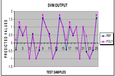
[image:5.612.83.265.333.386.2] [image:5.612.73.273.435.675.2] [image:5.612.75.273.516.571.2] [image:5.612.77.272.595.668.2]that SVM with polynomial kernel provides a good performance for prediction and classification [27]. Another study indicates that SVM with RBF kernel has stronger ability [14]. The classification accuracy results of test set of stroke risk prediction by SVMRBF and SVMPoly are shown in Table 10. It is also observed that the samples 1 and 16 are only misclassified (misclassification error is 0.08%) by using SVM Poly model, whereas in SVM RBF model, all samples (except the sample 22) of test set are correctly classified (misclassification error is 0.02%) is shown in Figure 1. The proposed models are well fit-in in the stroke risk prediction. The study proved and confirmed the validity of SVM kernels like RBF, and Poly. It also provided the good performance accuracy. It is believed that the SVC models have been suited for stroke risk prediction.
SVM OUTPUT
-1.5 -1 -0.5 0 0.5 1 1.5 2
1 3 5 7 9 11 13 15 17 19 21 23 25
TEST SAMPLES
P
R
E
D
IC
T
E
D
V
A
L
U
E
S
[image:6.612.81.267.232.355.2]RBF POLY
Figure 1. Two-class classification accuracies by SVMRBF and SVMPoly
machines
VI. CONCLUSION
In this study, the classification models are evaluated through SVMRBF and SVMPoly. The results strongly suggest that these models can assist the medical practitioners for planning the proper treatment strategies in the stroke risk prediction. We hope that more interesting results would be possible through further exploration of huge population data set. Authors conclude that the proposed prediction models would assist in the reduction of mortality and morbidity rate of stroke populations.
VII. REFERENCES
[1] Adams H, Adams R, Del Zippo G and Goldstein LB, Stroke Council of the American Heart Association; American Stroke Association. “Guidelines for the early management of patients with ischemic stroke: 2005 guidelines update: a scientific statement from the Stroke Council of the American Heart Association/American Stroke Association”, Stroke, 36: 916-923, 2005.
[2] Aszalos, Z, Barsi, P, Vitrai, J and Nagy, Z, “Hypertension and clusters of risk factors in different stroke subtypes”, Jr. of Human Hypertension, Vol.16, 495-500, 2002.
[3] Cathy M. Helgason, Thomas H Jobe, Casual interactions, Fuzzy sets and Cerebrovascular “Accident”: The limits of Evidence based medicine and the advent of complexity based medicine,
Neuroepidemiology, Vol.18, 64-74, 1999.
[4] Chao-Ton Su, Chien-Hsin Yang, “Feature selection for the SVM: An application to hypertension
diagnosis”, Expert Systems with Applications, Vol.34, 754-763, 2008.
[5] Cheng-Lung Huang, Hung-Chang Liao, Mu-Chen Chen, “Prediction model building and feature selection with support vector machines in Breast Cancer diagnosis”, Expert Systems with Applications, Vol.34, 578-587, 2008.
[6] Cortes, C., and Vapnik, V., Support vector networks machine learning, (pp.237-297). Boston, MA: Kluwar Academic Publisher, 1995.
[7] De Beule M, Maes, E, De Winter, O, Vanlaere, W, Van Impe, R., “Artificial Neural Networks and risk stratification: A promising combination”,
Mathematical and Computer Modeling, Vol.46, 88-94, 2007.
[8] Emre Comak, Ahmet Arslan, Ibrahim Turkoglu, “A decision support system based on support vector machines for diagnosis of the heart valve diseases”,
Computers in Biology and Medicine, Vol.37, 21-27, 2007.
[9] Gorelick PB. (1995). Stroke prevention. Arch. Neuro., Vol.52: 347-355, 1995.
[10]Ioannis Nomikas, Georgios Dounias, Georgios Tselentis, Konstantinos Vemmos, “Conventional Vs. Fuzzy modeling of diagnostic attributes for classifying acute stroke cases”, ESIT (European Symp. On Intelligent Techniques), 14-15 September, 2000, pp.192-200, 2000.
[11]Jeyavatdhana Rama, G.L., Alistair P. Shilton, Michael M. Parker, and Marimuthu Palaniswami, “Prediction of cystine connectivity using SVM”,
Bioinformation 1(2): 69-74, 2005.
[12]Kemal Polat, Salih Gunes, Ahmet Arslan., “A cascade learning system for classification of diabetes disease: Generalized Discriminant Analysis and Least Square Support Vector Machine”, Expert Systems with Applications, Vol.34, 482-487, 2008.
[13]Lisboa, P.J., “A review of evidence of health benefits from Artificial Neural Networks in medical intervention”, Neural Networks, 15(1): 11-39, 2002.
[14]Lukas, L., Devos, A., Suykens, J.A.K. Vanhamme, L., Howe, F.A., Majos, C., et.al., “Brain tumor classification based on long echo proton MRS signals”. Artificial Intelligence in Medicine. 31, 73-89, 2004.
[15]Mosalov, O.P., Rebrova, O. Yu, and Red’ko, V.G., “Neuroevolutionary Method of Stroke Diagnosis”,
Optical Memory and Neural Networks (information optics), Vol.16, No.2, 99-103, 2007.
[16]Murphy, C.K., “Identifying diagnostic errors with induced decision trees”. Medical Decision Making, 21(5), 368-375, 2001.
[17]Olga REBROVA, Valery KILIKOWSKI, Sofia OLIMPIEVA, Oleg ISHANOV, “Expert system and Neural Network for stroke diagnosis”, Intl. Jr. of Information Technology and Information Communication, Vol.2, No.1, 441-452, 2006.
Cerebrovascular Diseases, Vol.15, No.5, 223-227, 2006.
[19]Renke Maas., Rainer H Boger, “Old and new cardiovascular risk factors: from unresolved issues to new opportunities”. Atherosclerosis Supplements
4, 5–17. PMID: 14664897, 2003.
[20]Sabibullah, M. Kasmir Raja S.V., “A Neural prognostic model for predicting stroke prone risk factors”, Bio-Science Research Bulletin, Vol.23(2), 95-102, 2007.
[21]Spitzer, K, Thie, A, Caplan, LR, and Kunze K., “The MICROSTROKE expert system for stroke type diagnosis”, Stroke, 20; 1353-1356, 1989.
[22]Stephen R. Alty, Sandrine C. Millasseau, Philip J.
Chowienczyk and Andreas Jakobsson,
“Cardiovascular disease prediction using Support Vector Machines”, Circuits and Systems (MWSCAS; 03), Proc. of the 46th IEEE Intl., Midwest Symp. On..Vol.1, 376-379, 2003.
[23]homas Lumley, Richard A. Kronmal, Mary Cushman, Teri A. Manolio, Steven Goldstein, “A stroke prediction score in the elderly: Validation and Web-based application”, Journal of Clinical Epidemiology, Vol.55, 129-136, 2002.
[24]Tjortjis, C. Saraee, M, Theodoulidis B, and Keane, J.A., “Using T3, an improved Decision Tree classifier, for mining stroke related medical data”,
Methods of Information in Medicine, Vol.46(5), 523-529, 2007.
[25]Tsujinishi, D., and Abe, S., “Fuzzy least squares SVM for multi-class problems”. Neural Networks field (Vol.16). Elsevier (pp.785-792), 2003.
[26]Vapnik, V.N., Statistical learning theory. New York: Wiley – Inter Science, 1998.
[27]Wang, M.L., Li, W.J., and Xu, W.B., “Support vector machines for prediction of peptidyl prolyl