Towards high velocity deformation characterisation of metals
and composites using Digital Image Correlation
R. Eriksen1, C. Berggreen1, S. W. Boyd2, J.M. Dulieu-Barton2
1
Department of Mechanical Engineering, Technical University of Denmark, Nils Koppels Allé, 2800 Kongens Lyngby, Denmark
2
School of Engineering Sciences, University of Southampton, Highfield, Southampton, SO17 1BJ United Kingdom
Abstract
Characterisation of materials subject to high velocity deformation is necessary as many materials behave differently under such conditions. It is particularly important for accurate numerical simulation of high strain rate events. High velocity servo-hydraulic test machines have enabled material testing in the strain rate regime from 1 – 500 ε/s. The range is much lower than that experienced under ballistic, shock or impact loads, nevertheless it is a useful starting point for the application of optical techniques. The present study examines the possibility of using high speed cameras to capture images and then extracting deformation data using Digital Image Correlation (DIC) from tensile testing in the intermediate strain rate regime available with the test machines. Three different materials, aluminium alloy 1050, S235 steel and glass fibre reinforced plastic (GFRP) were tested at different nominal strain rates ranging from quasi static to 200 ε/s. In all cases DIC was able to analyse data collected up to fracture and in some cases post fracture. The use of high-speed DIC made it possible to capture phenomena such as multiple necking in the aluminium specimens and post compression failure in GFRP specimens.
1 Introduction
High speed tensile tests at intermediate strain rates up to 500 ε/s are accessible with high speed servo-hydraulic test machines [1]. Available commercial test machines can achieve test velocities of 20-25 m/s controlled in open loop mode. For homogeneous material the use of “dog bone” shaped specimens is possible, and if the strain rate is below 10 ε/s the load can be measured using piezo
-electric load cells. Above 10 ε/s the load is measured with local force transducers to suppress the effect of load cell ringing [2, 3]. For heterogeneous materials, such as fibre reinforced polymer composites, it is generally necessary to use straight sided strip specimens. Local force transducers require that a portion of the specimen remains linear elastic which is difficult to control with the strip
specimens. Therefore it is necessary to use a piezo electric load cell for all strain rates with a strip specimen.
Strain is normally measured with extensometers up to around 1 ε/s. For strain rates higher than 1 ε/s strain gauges or high speed non-contact measurement methods such as laser Doppler
© Owned by the authors, published by EDP Sciences, 2010 DOI:10.1051/epjconf/20100631013
EPJ Web of Conferences
extensometers can be used [4]. All extensometers provide the average strain within the measured gauge length whereas a strain gauge measures the average strain within the associated measuring grid. Strain gauges can generally be used at all strain rates, however correct adhesive selection is a major consideration to ensure the gauge does not debonding from the specimen.
The application of Digital Image Correlation (DIC) to images obtained from high speed cameras provides full-field strain data. Local variation in strain can be obtained, as well as the average strains across a pre-defined area similar to that obtained with an extensometer. The use of imaging means there are no difficulties with gauge attachment and local reinforcement. Additionally, the acquisition of full-field data enables local strains to be determined including the failure initiation and the damage progression to be captured. If the images are processed using DIC, the component strains can be extracted and related to the failure. The full-field capability of DIC is particularly important for composite materials, where failure mechanisms are complex and the point of initiation undefined. The present paper provides some guidelines for application of DIC to data captured from high speed imaging of specimens of different materials loaded in a high-velocity servo-hydraulic test machine. Stress-strain curves are produced based on simultaneous measurement of load with image capture at different test velocities that demonstrate the feasibility of using the DIC approach for material characterisation.
2 High-speed DIC using ARAMIS
2.1 Displacement and strain calculationTo obtain the images two Photron APX-RS high speed cameras are used, which can achieve 3000 frames per second (fps) at full resolution of 1k x 1k pixels with a 10 bit resolution. By windowing it is possible to achieve up to 250000 fps over at 128 x 16 pixels. The cameras have a memory capacity of 8 GB. Therefore a choice must be made between temporal resolution (fps) and spatial resolution as well as the displacement range over which images are captured [5]. For material characterisation at different strain rates, recommendations in relation to data sampling rates are defined by ISO/DIS
26203-2 for metals [2], and provide a basis for assessing camera capabilities in terms of image capture rates. Standards for high-speed characterisation of composite materials are not available. There is an SAE standard for polymers [6], but does not provide sampling rates. In [2] the following sampling rate for strain and load measurements is recommended:
(1)
where is the nominal strain rate calculated from the test velocity and the gauge length.
To apply DIC successfully the minimum feasible spatial resolution of the Photron APX-RS cameras for DIC is 256 x 32 pixels. The frame rate is therefore limited to 112500 fps, which according to equation (1) means a maximum strain rate of only 28 ε/s can be applied. This may not be sufficient for certain materials, so it may be necessary during imaging to increase the spatial resolution of the camera and only sample the load data at the required frequency. This is not ideal, but part of the trade off between spatial and temporal resolution dictated by the camera capabilities. In the cases where the image sampling is insufficient the strain data can be interpolated by using the load data and thereby making the assumption of a constant strain rate. It is appreciated in these cases that the derived strain may not be accurate, e.g. yield points for metals. The minimum temporal resolution, and thus the maximum camera sampling rate, should be chosen by establishing the number of pixels required in the image for the DIC data processing. To do this successfully a number of variables related to the DIC processing require consideration; these are discussed below.
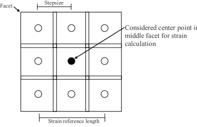
movement of the greyscale distribution within each facet relative to its centre point from image to image to obtain a displacement. Furthermore, adjacent facets are spaced with a distance denoted step sizewhich can be smaller than the facet size resulting in overlapping facets, see Figure 1. Once the facet centre point displacement vectors have been determined, the strain can be obtained. The commercial DIC system, ARAMIS [7], used in this work uses a square field of a minimum of 3 x 3 facet centre points to calculate the strain at the considered facet centre point. The number of centre points used in the strain calculation is denoted computation size in the ARAMIS software, e.g a strain computation size of 5 means using a field of 5 x 5 centre points. For an edge facet the strain tensor can still be calculated by using only 5 neighbouring points [8]. The neighbouring centre points displacements are used to estimate the average deformation gradient over a gauge length
defined by the facet step size and the computation size according to Figure 1 and hence the 2D strain tensor is obtained. For a step size of 5 pixels and computation size of 3 the strain reference length
would be 10 pixels.
Fig. 1 Local 3x3 space for calculation of the strain tensor
The facet size directly determines the spatial resolution of the displacements and strains, since the greyscale information within a facet is used for the correlation between images. Furthermore, larger facet sizes will result in better accuracy of the image correlation. The step size will in conjunction with the computation size directly determine the strain reference length, see Figure 1. Generally, the step size should always be less than the facet size to maximise the use of the information in the image. However, it will be meaningless to use a step size of 1 pixel since the inaccuracies in facet centre point positions will be a large fraction of the strain reference length. In each application it should be considered if the average strain over a number of facets or the strain variation facet by facet is most important. The resultant is another trade off in this case between
spatial resolution (smaller facet sizes) and strain precision (larger facet sizes). Here because of the
need to maximise the high speed camera temporal resolution, local strain variations were considered to be of secondary priority and consequently the low resolution images were accepted.. Given the limited resolution of the images a step size was chosen of 5 pixels for a facet size of 15 pixels to give more than one facet across the test specimens width. With a window of 256 x 32 pixels there is space for 3 centre points across the specimen. For comparison, the default settings in ARAMIS are 13 pixels for step size and 15 x 15 pixels for the facet size.
For ARAMIS a rough estimate of the accuracy is 1/30 pixel for the facet centre point positioning [5]. However, with careful camera calibration and a good speckle pattern the accuracy can be as good as
1/100 pixel. Assuming a constant uniaxial strain field, the maximum error in the displacement between two centre points will be twice the inaccuracy in a single facet centre point positioning, i.e.
1/15 pixel. For a strain reference length of for example 10 pixels this corresponds to of 0.67% strain, and would be the maximum noise that occurs due to measurement uncertainties. 0.67% strain uncertainty is clearly unacceptably high. However this can be mitigated by assuming a uniform strain in the specimen and obtaining the average strain from all the facets. Alternatively, the system
Stepsize
Strain reference length
EPJ Web of Conferences
can be used as a video extensometer and the strain calculated between two facet centre points placed at a certain distance from each other. The latter case was used in the present work, as this gave a greater strain reference length of 100 to 180 pixels, resulting in a a better signal to noise ratio. Using
180px gives a maximum noise of 0.03%. It is clear from the above discussion that a window size of
256 x 32 pixel will give noisy local strain measurement due to small strain reference lengths and effects from edge facets which is affected be fewer neighbouring points for estimation of the strain tensor.
2.2 Speckle patterns
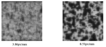
In general the random pattern required for DIC is created in the form of a spray paint speckle, where an individual speckle should be cover at least 3 x 3 pixels [5, 9]. If the spatial resolution of the camera is changed the number of pixels per mm will change and the physical speckle size must be
adjusted accordingly. However, if the speckles are too small they will be covered by very few pixels and the transition from black to white and opposite will be smoothed, leading to low contrast in the image and thus reduced accuracy of the image correlation [9]. This is shown in Figure 2 where two speckle patterns are captured at different image magnification factors, Mt. An alternative approach to the random pattern is to generate a regular pattern. The ARAMIS correlation algorithms are able to use regular patterns [8] by limiting the maximum displacement of the facets between images [10, 11] to be less than the period of the pattern to avoid aliasing. Furthermore, the facet size relative to the period of the pattern should also be sufficiently small so that a displacement equal to the facet size is
required before a facet is repeated over the pattern. Additionally, the individual facets must not be smaller than the pattern period. Usually there is a slight greyscale distribution at the transitions in the regular pattern and that has a positive effect on both facet registration and correlation. This is particularly important for data collected at the margins of the recommendations mention above.
Figure 4 shows the speckle patterns used in this study. Pattern (a) was created with spray paint and during imaging a resolution of 7.58 pixel/mm was used. Pattern (b) was created with a felt tip
pen with a pen size of 1.5 mm and in imaging gave 3.86 pixel/mm. Pattern (c) was created with a stencil and spray paint to produce regular black circles of 2 mm in diameter with a 4 mm pitch from centre to centre to give 2.35 pixel/mm.
Fig. 2 Impact of image magnification on sampling of
stochastic speckle patterns Fig. 3 Different speckle patterns with super imposed facet
For resolutions of less than 3.5 - 4.5 pixel/mm it was difficult to create a high contrast random speckle pattern with spray paint. Therefore it was decided to test the regular patterns that are typically used for large FOV’s in structural testing, e.g. [11] as the regular patterns could be applied more consistently between specimens.
[9]. At this stage the paint had sufficient elasticity which was especially important with steel specimens where uniform strains up to 10% were encountered.
2.3 Calibration
When using a HS camera with limited resolution, the calibration must always be carried out at full resolution [5]. ARAMIS uses a rectangular calibration panel with circular markers of know size and
spacing defining a 3D measurement volume. This allows the displacement distance to be defined both in-plane and out-of plane. The minimum window of 256 x 32 used in this work covers 65 x 12
mm to give a pixel magnification factor of 4 px/mm. Using a window size of 256 x 256 px for calibration will give a FOV of 65 x65 mm but the markers on the calibration panel for this size will
only be covered by 4 x 4 pixels, making an accurate positioning of the marker centres impossible resulting in an imprecise calibration. Therefore it was necessary to use the full FOV of 260 x 260 mm at 1024 x 1024 pixels with an appropriate calibration panel. The quality of the calibration is measured in the pixel deviation factor and should generally be lower than 0.04 pixels and in this work all calibrations was better than 0.03px.
2.4 Shutter time and blur
The amount of blur depends on MT, the velocity of the object in reference to the image sensor (V) and the integration time (te). A relation for the amount of blur can be expressed as [9]:
(2)
ARAMIS can handle blur up to 1 pixel [12]. However for the present study the limit of blur in relation to calculating the maximum integration time for a given setup was set to 0.25 pixels. It should be noted in connection with the estimation of the velocity of the specimen that the velocity field is not constant along the specimen when subjected to a constant strain rate, thus a qualified estimation must be adopted. Additionally, it may also be necessary to use even shorter integration times to avoid blur in circumstances such as rapid cracking of composite materials.
2.5 Illumination
Illumination of the sensor must be optimized to maximise the use of the maximum range of greyscale available in the images [9]. Although the Photron cameras have a 10 bit resolution the Aramis system works on an 8 bit range therefore a greyscale range of 0 to 255 is available however working to full saturation is not recommended as this often results in data loss so 20 to 230 was considered to be a good operating range.. When a stereo setup is used it is important to obtain an equal illumination in both cameras. As mentioned in the previous section the integration time will be a few µs for high test velocities to avoid blurring. Therefore to obtain the necessary contrast within the 8 bit range significant of illumination is necessary which was obtained with by using high power halogen lamps. It should be noted that these lamps can heat the specimen so they were only used when the images were collected to minimise the heat exposure, even so [6] this could affect the measured material properties.
3 Test setup
EPJ Web of Conferences
of material with end tabs. Steel S235 specimens of 50 mm working length, 10 mm wide and 2.8 mm thick, and aluminium alloy specimens of 50 mm working length, 8 wide and1.0 mm thick and E-glass/epoxy composite cross-ply [0/90]6s of 100 mm long by 25mm wide and 2.1mm thick were
manufactured and tested at 6 nominal strain rates from quasi-static to 200 ε/s. The steel specimens
had a single Vishay BG250 strain gauge bonded in line with the specimen longitudinal axis. The Vishay AE15 epoxy adhesive was used as this can withstand strains up to 15%. A Vishay 2311 amplifier was used for conditioning of the strain gauges. The GFRP specimens were equipped with a Vishay 240UZ strain gauge and the aluminium alloy specimen was equipped with a HBM 1-LY11 strain gauge.
An Instron VHS 80/20 (80 kN and 20 m/s) high-speed servo-hydraulic test machine running in
open loop was used for tests above 1 m/s. Below 1 m/s a modified MTS 810 155 kN servo-hydraulic test machine was used running in closed loop control. Load levels were measured with a piezo -electric load cell and local force transducers for the high-speed tests above 1 m/s, and with a conventional MTS 250 kN load cell for low speed tests below 1 m/s. The two Photron APX-RS cameras were positioned so that they shared the same vertical axis and viewed the specimen at an angle of approximately 25°. The ARAMIS system software was used to control and synchronise the image acquisition from both cameras. The stereo setup (3D) allowed the out of plane deformation to be computed using 3D DIC image processing. Both speckle and regular patterns were created as described above. The speckles had sizes between 3-6 pixels and the magnifications factors were between 8.53 pixels/mm and 2.35 pixels/mm depending on the applied frame rate.
4 Results
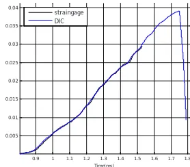
Figure 4 shows the “DIC” strain value calculated from the average strain across the necking region of a steel specimen and the “DIC 8 mm” value from an area of length equivalent to that of the strain gauge, but away from the necking region. This clearly shows the benefit of the local measurement possible with the full-field DIC approach. In Figure 5 for a GFRP specimen it is seen that the strain gauge signal is lost before the DIC signal, due to debonding of the gauge. Generally with composite specimens the strain gauge debonded at fracture when the elastic energy was released, while the imaging could be extended into the post-failure regime. It is useful to compare the Young’s modulus, E, obtained from the strains provided by the DIC and strain gauge measurements. The mean and standard deviation were calculated for the difference E (Strain gauge) – E (DIC) for all specimens and are provided in Table 1. The Pvalue is the probability that the difference is equal to zero. Thus
these results show the ability of DIC for use in material characterizations by adopting appropriate patterns for the different image magnifications across all test velocities. It is important to emphasise here that the values quoted in Table 1 are average values obtained from different patterns and frame rates, the values of which are given in Table 2.
A selected full-field DIC contour plot is shown in Figure 6, where two necking regions were found on an aluminium specimen. A similar mechanism was found at four specimens at 45 ε/s,
illustrating that DIC can capture phenomena that strain gauge cannot.
Table 1 - Comparison of measured E moduli from DIC and strain gauge measurements.
Steel GFRP Aluminium 1050
Mean E Strain gauge 203.8 17.80 57.52
Mean E DIC 213.0 17.42 59.61
Mean of difference -6.415 0.3733 -2.090
95% Confidence interval -12.52 to -0.3120 0.05108 to 0.6956 -6.162 to 1.982
Fig. 4 Steel 10m/s – 162 ε/s Fig. 5 GFRP 20m/s - 45 ε/s
Fig. 6 A full-field DIC major principal strain plot showing multiple necking regions in an aluminium specimen at 45 ε/s.
Table 2 – Example of image sizes and magnifications factors for steel
Nominal strain rate (ε/s) 0.00025 2 10 100 200
Frame rate 1 10000 50000 112500 112500
Images size (pixel) 2048x2038 640x128 512x96 256x32 256x32
Magnification factor (pixel/mm) 21 8.53 7.58 3.86 3.86
Speckle pattern Stochastic Stochastic Stochastic Felt tip pen Felt tip pen
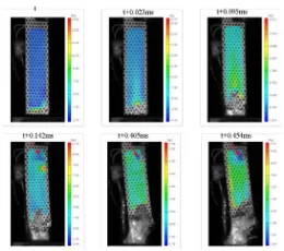
Despite the small P values the mean differences in Table 1 are only small fractions of the measured E values, and the small differences were therefore found to be acceptable. However, it should be noted that strain gauge measurements can be affected by measurements errors as well and with 3D DIC it is also possible to account for out of plane motion. In general strain variations for all tested specimens were consistent with those presented in Figures 4 and 5. It was also noticed that only a single steel specimen out of 22 specimens fractured within the area of the strain gauge. Furthermore, the use of solder terminals were avoided because they affected the deformation behavior in the plastic region as shown in Figure 7. The results in Figure. 7 also indicate that the use of strain gauges themself affects the material behaviour. Here DIC has an advantage since the applied paint for the speckle pattern is less stiff than a strain gauge and is applied to the entire surface of the specimen. Finally, compression damage was found on many GFRP specimens and it was possible to follow the build-up of the compressive stresses as shown in Figure 8.
5 Conclusions
Some initial work on the application of DIC to the derivation of strains from metallic and composite specimens subjected to high speed deformation has been presented. The work includes some
1 1.1 1.2 1.3 1.4 1.5 1.6 1.7
0.02 0.04 0.06 0.08 0.1 0.12 0.14 0.16
Time(ms)
ε
straingage DIC DIC 8mm
0.9 1 1.1 1.2 1.3 1.4 1.5 1.6 1.7 1.8 0.005
0.01 0.015 0.02 0.025 0.03 0.035
Time(ms)
ε
EPJ Web of Conferences
noteworthy findings that will provide guidance for other practitioners, It should be noted that the DIC system used to control the acquiring and the processing of the data was the ARAMIS system by GOM and some of the features discussed in the paper are only applicable to this system. Most importantly in this regard is the ability for the system to cope with a regular pattern for correlation, which was particularly useful for consistent marking of the specimens. A pair of Photron APX-RS high-speed cameras was used to collect the image data for the DIC from specimens loaded in two high velocity testing machines. The work shows that spatial resolution can be sacrificed to allow increased temporal resolution by averaging of the strains determined from the DIC across the specimen. The strain data extracted from the DIC were still able to assess the variation of strain across the gauge length, making it possible to identify effects such as multiple necking regions and post-failure compression regions. The guidelines presented in this paper and the results achieved illustrate that the use of DIC can add valuable insight into high strain rate material failure, which cannot be obtained with conventional strain gauge measurements.
Fig. 7 Influence on deformation behaviour from strain gauge and solder terminals.
Fig. 8 Compression in GFRP specimen after main
fracture at a strain rate of 40 ε/s. The colour field
represent major strain and the scale bar is adjusted for each image. The red arrows indicate regions of compression strains. The sequence was captures at
42.000 fps.
6 References
1. Bardenheider R, Rogers G Dynamic Impact Testing. Instron(2003)
2. ISO-CD2 26203-2.2 Metallic Materials - Tensile Testing method at high strain rates - Part2: Servo-Hydraulic and other test systems, 2nd edn. ISO(2008)
3. Wood PKC, Burkley M Strain Rate Testing of Metallic Materials and their Modelling for use in CAE based Automotive Crash Simulation Tools (Recommendations & Procedures). Warwick University(2008)
4. High Strain Rate Experts Group Recommendations for Dynamic Tensile Testing of Sheet Steels. International Iron and Steel Institute(2005)
5. Schmidt T, Tyson J, Galanulis K, Revilock D, Matthew M 26th International Congress on High-Speed Photography and Photonics 5580:174-185(2004)
6. SAE Standard: J2749 High Strain rate Tensile Testing of PolymersSAE (ed) . SAE(2008)
7. GOM ARAMIS. In: . http://www.gom.com/EN/deformation.measurement/material.testing/material.properties.html. Accessed 10/30 2009
8. GOM ARAMIS - User Manual - Software. Ver. 6.1. GOM(2007)
9. M. A. Sutton Image Corrolation for Shape, Motion and Deformation Measurements Basic Concepts, Theory and Applications. Springer(2009)
10. Helm J . Exp Mech 48:753-762(2008)
11. Helm J, Kurtz S, Salkini A, O'Brien E . The Journal of Strain Analysis for Engineering Design 43:761-768(2008) 12. Mail correspondence with GOM (2010)