157 |
P a g e
www.ijarse.com
ANALYSIS OF IMPORTANCE SAMPLING AND
CONTINGENCY IN ELECTRIC POWER SYSTEM
SECURITY
Nandini.BR
1, Dr. R. Prakash
2, Mrs. Lekshmi.M
31
P.G student, Department of Electrical and Electronics Engineering ,
Acharya Institute of Technology, V.T.U, Belgaum, Karnataka, (India)
2
Professor, Department of Electrical and Electronics Engineering,
Acharya Institute of Technology, V.T.U, Belgaum, Karnataka, (India)
3
Associate Professor, Department of Electrical and Electronics Engineering,
Acharya Institute of Technology, V.T.U, Belgaum, Karnataka, (India)
ABSTRACT
Power system security has become one of the most important issues in power system operation due to intensive use of transmission network and it is strongly tied with contingency analysis. However with the introduction of more variable generation sources such as wind power and due to fast changing loads power system security analysis will also have to incorporate sudden changes in injected powers that are not due to generation outages. The probability of failure induced by changes in grid state is evaluated by the Monte Carlo simulation method. A comparison to crude Monte Carlo (CMC) and Importance sampling (IS) method is performed for standard IEEE-33 bus system. Importance sampling method indicates a major increase in simulation efficiency by reducing number of samples.
Keywords:
Contingency, Crude Monte Carlo Method, Importance Sampling, Particle Swarm
Optimization, Power System Security.
I INTRODUCTION
Power system stability has been recognized as an important problem for secure system operation since the 1920s
[1]. In order to maintain the reliability of an electric power system at an appropriate level and at low cost, it is
essential that voltage stability be accurately assessed. There are a number of methods for assessing voltage
stability. There is a large conflict of interest between the market perspective, where a large capacity to transfer
power through the electric power grid is required, and the security perspective, where secure operation is the
main objective. To satisfy both objectives to the largest possible extent, an adequate balance between security
and capacity is preferable. This, in turn, calls for an efficient method for evaluating the security of a certain
operating state. With the introduction of large amounts of wind power, which is a more variable energy source
than conventional hydro-, nuclear-, and heat-power plant generation, more concern has to be put to the
158 |
P a g e
As a stable operating point of the power system drifts, it may eventually change its properties and becomeunstable; clearly this is a situation the system operator would like to avoid. To use an electric power system in
an efficient and reliable way, several issues will have to be considered. One of these issues is voltage stability. It
will be of great importance to keep the operating point within the stable domain, or else instability will occur,
leading to undesirable events such as system blackout. The main attention has been put to outages in the grid or
in the production units. In evaluating the probability of failure induced by changes in grid state, there are two
popular methods: the contingency enumeration method and the Monte Carlo simulation method.
The contingency enumeration method enumerates all contingencies that are considered plausible and analyses
the severity of each contingency. One example of such a method is the N-1-criterion [9], which states that the
system should remain stable after losing any single component. Hence, according to the N-1-criterion, the
contingencies that are considered plausible are all the contingencies where one component in the system fails,
and all contingencies with more than one failure are considered to have such a small probability of occurring
that they can be neglected in a security analysis of the power system. As the size of the system increases, so
does the risk of failure of multiple components in the system within a short time-frame. Therefore, methods for
identifying high risk N-K contingency situations were suggested in [3].
A contingency not leading to immediate loss of stability may still reduce stability margins so that a plausible
change in injected power following a contingency leads to instability before preventive measures have time to
take effect. Whether one uses the contingency enumeration method or the Monte Carlo method to generate the
state of the grid and the generating units, some concern will, thus, also have to be taken to the change in
operating conditions induced by change of loads or change in production in more variable production units like
wind- or wave-power plants.
One technique that has been applied successfully in stochastic analysis of dynamic systems of high dimension is
the double and clump (D&C) [8] method. D&C provides a means to increase the number of samples which are
expected to contribute to the estimation of low probability regions. In analogy to the importance sampling
technique, these contributing samples are considered as important samples. The increase of the important
samples is carried out by the doubling procedure. To keep the sample size constant, from the viewpoint of
computational efficiency, the number of less important samples is reduced through the clumping procedure.
Unfortunately this method requires heuristic knowledge of which sample values that is important and should be
doubled and which that are not so important and can be clumped. Therefore, it is not that suitable in power
system security evaluation.
II PROBLEM FORMULATION
In power system operation, there are number of stable operation criteria that have to be fulfilled at all times.
159 |
P a g e
www.ijarse.com
2.1
Voltage Stability
There must for each set of injected power p exist a vector such that the power flow equations, f(x, p) =0 are
fulfilled. Furthermore, the operating point (x, p) must always be a stable operating point, so that after any small
change in operating conditions, the system returns to stable operation.
2.2
Thermal Stability
Due to limitations in the power system equipment, some of the equipment such as power-lines will be
disconnected if the current flowing through the equipment becomes too large. Therefore, the electric power
transfers in the system cannot be allowed to exceed some set maximal value.
2.3
Voltage Limits
The voltages at certain nodes might have to be kept within a predefined interval.
2.4 Optimal placement of DG in distribution network problem is to minimize the real power losses and improve
the voltage profile, which is calculated as follows:
𝐹1 𝑋 = 𝑃𝐿 = 𝑁𝑏𝑟𝑅𝑖𝐼𝑖2 (1)
𝑖=1
Where, Ri and Ii are resistance and actual current of the ith branch, respectively. Nbr is the number of the
branches.
III MONTE CARLO METHOD
Monte Carlo methods provide approximate solutions to a variety of mathematical problems by performing
statistical sampling experiments. They can be loosely defined as statistical simulation methods, where statistical
simulation is defined in quite general terms to be any method that utilizes sequences of random numbers to
perform the simulation. Thus Monte Carlo methods are a collection of different methods that all basically
perform the same process. This process involves performing many simulations using random numbers and
probability to get an approximation of the answer to the problem. Thus the analysis of the approximation error is
a major factor to take into account when evaluating answers from these methods. The attempt to minimize this
error is the reason there are so many different Monte Carlo methods. The various methods can have different
levels of accuracy for their answers, although often this can depend on certain circumstances of the question and
so some method’s level of accuracy varies depending on the problem. Different types of Monte Carlo methods
are
Crude Monte Carlo
Acceptance-rejection Monte Carlo
Stratified sampling
Importance sampling
This is illustrated well in the [12]. In this paper CMC and IS method is implemented with the numerical
example of IEEE-33 bus system, and compare their answers in terms of number of sample and the accuracy of
160 |
P a g e
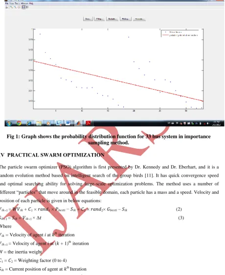
Fig 1: Graph shows the probability distribution function for 33 bus system in importance
sampling method.
IV PRACTICAL SWARM OPTIMIZATION
The particle swarm optimizer (PSO) algorithm is first presented by Dr. Kennedy and Dr. Eberhart, and it is a
random evolution method based on intelligent search of the group birds [11]. It has quick convergence speed
and optimal searching ability for solving large-scale optimization problems. The method uses a number of
different “particles” that move around in the feasible domain, each particle has a mass and a speed. Velocity and
position of each particle is given in below equations:
𝑉𝑖𝑘+1 = 𝑊𝑉𝑖𝑘 + 𝐶1 × 𝑟𝑎𝑛𝑑1 × 𝑃𝑏𝑒𝑠𝑡𝑖 − 𝑆𝑖𝑘 + 𝐶2 × 𝑟𝑎𝑛𝑑2× 𝐺𝑏𝑒𝑠𝑡𝑖 – 𝑆𝑖𝑘 (2)
𝑆𝑖𝑘+1 = 𝑆𝑖𝑘 + 𝑉𝑖𝑘+1 × Δ𝑡 (3)
Where
𝑉𝑖𝑘 = Velocity of agent i at 𝑘th iteration
𝑉𝑖𝑘+1 = Velocity of agent i at (𝑘 + 1)th iteration
W = the inertia weight
𝐶1 = 𝐶2 = Weighting factor (0 to 4)
𝑆𝑖𝑘 = Current position of agent at 𝑘th Iteration
𝑆𝑖𝑘+1 = Current position of agent at (𝑘 + 1)th Iteration
𝑖𝑡𝑒𝑟𝑚𝑎𝑥 = Maximum iteration number
𝑟𝑎𝑛𝑑1, 𝑟𝑎𝑛𝑑2 = the random numbers selected between 0 and 1.
𝑃𝑏𝑒𝑠𝑡𝑖 = 𝑃𝑏𝑒𝑠𝑡 of agent i
161 |
P a g e
www.ijarse.com
Δ𝑡 is change in time step from two successive iterations.
The PSO-based approach for solving optimal placement of distributed generation (OPDG) problem to minimize
the loss takes the following steps; flow chart is shown in figure 2
Step 1: Input line and bus data, and bus voltage limits.
Step 2: Calculate the loss using Newton’s Raphson method.
Step 3: Randomly generates an initial population (array) of particles with random positions and velocities on
dimensions in the solution space. Set the iteration counter k=0.
Step 4: For each particle if the bus voltage is within the limits, calculate the total loss. Otherwise, that particle is
infeasible.
Step 5: For each particle, compare its objective value with the individual best. If the objective value is lower
than Pbest, set this value as the current Pbest, and record the corresponding particle position.
Step 6: Choose the particle associated with the minimum individual best Pbest of all particles, and set the value of
this Pbest as the current overall best Gbest.
Step 7: Update the velocity and position of particle.
Step 8: If the iteration number reaches the maximum limit, go to Step 9. Otherwise, set iteration index k=k+1,
and go back to Step 4.
Step 9: Print out the optimal solution to the target problem. The best position includes the optimal locations and
size of, DG, and the corresponding fitness value representing the minimum total real power loss.
Figure 2: Flow chart of PSO
No
End
Update particle position and velocity (7)
Check the stopping criteria
(8)
Calculate the original loss using NR method (2)
Initialize particle population (3)
Calculate the total loss (4)
Record Pbest (5), Gbest(6)
Start
Input system data (1)
Print out location of the DG (9)
162 |
P a g e
V CONTINGENCY SELECTION
Contingency analysis process involves the prediction of the effect of individual contingency cases, the process
becomes very tedious and time consuming when the power system network is large. In order to alleviate the
above problem contingency screening or contingency selection process is used. The process of identifying the
contingencies that actually leads to the violation of the operational limits is known as contingency selection. The
contingencies are selected by calculating a kind of severity indices known as Performance Indices (PI). These
indices are calculated using the conventional power flow algorithms for individual contingencies in an off line
mode. Based on the values obtained the contingencies are ranked in a manner where the highest value of PI is
ranked first. The analysis is then done starting from the contingency that is ranked one and is continued till no
severe contingencies are found.
There are two kind of performance index which are of great use, these are active power performance index (PIP)
and reactive power performance index (PIV). PIP reflects the violation of line active power flow and is given
below:
𝑃𝐼𝑝 =
(𝑃𝑖/𝑃𝑖𝑚𝑎𝑥)
2𝑛
(4)
𝐿
𝑖=1
Where
Pi = Active Power flow in line i
Pimax= Maximum active power flow in line i
n is the specified exponent
L is the total number of transmission lines in the system.
If n is a large number, the PI will be a small number if all flows are within limit, and it will be large if one or
more lines are overloaded. Here the value of n has been kept unity. The value of maximum power flow in each
line is calculated using the formula:
P
imax= (Vi*Vj)/X (5)
Where,
Vi= Voltage at bus i obtained from NR solution
Vj= Voltage at bus j obtained from NR solution
X = Reactance of the line connecting bus “I” and bus “j”
Another performance index parameter which is used is reactive power performance index corresponding to bus
voltage magnitude violations. It mathematically given in equation 6:
163 |
P a g e
www.ijarse.com
Where
Vi= Voltage of bus i
Vimax and Vimin are maximum and minimum voltage limits Vinom is average of Vimax and Vimin
Npq is total number of load buses in the system flow chart for contingency selection technique is shown in Fig. 3
Figure3: Flow chart of contingency selection
End Compute PIp & PIv
Last outage done? Set the counter to simulate
contingency
Simulate the line outage contingency
Run the load flow analysis for this outage condition
Start
Initialize & read the system variables
variable
Sort PIp & PIv values and rank them
Select high PIp & PIv values and classify it as critical contingency
case
No
164 |
P a g e
VI NUMERICAL EXAMPLE
In this section, a numerical example will be presented. The aim of the numerical example is to show the
efficiency of the importance sampling technique proposed in this paper. The calculations will be performed on
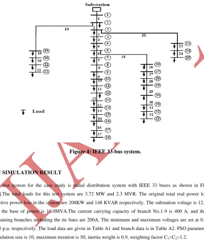
the IEEE 33-bus system depicted in fig-4.
Figure 4: IEEE 33-bus system.
VII SIMULATION RESULT
The test system for the case study is radial distribution system with IEEE 33 buses as shown in Figure 4
[13].The total loads for this test system are 3.72 MW and 2.3 MVR. The original total real power loss and
reactive power loss in the system are 208KW and 148 KVAR respectively. The substation voltage is 12.66 KV
and the base of power is 10.0MVA.The current carrying capacity of branch No.1-9 is 400 A, and the other
remaining branches including the tie lines are 200A. The minimum and maximum voltages are set at 0.95 and
1.05 p.u. respectively. The load data are given in Table A1 and branch data is in Table A2. PSO parameters are,
population size is 10, maximum iteration is 50, inertia weight is 0.9, weighting factor C1=C2=1.2.
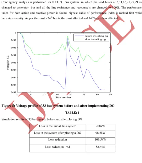
The improvement in the voltage profile after optimally placing the DGs is shown in Figure 5. Without DG, the
bus no. 18 has the lowest voltage of 0.923p.u. and the bus voltage has improved to 0.975p.u. after installing DG.
For the 33 bus system, as shown in table 1, the PSO can obtain the loss reduction. That is DG can reduce the
165 |
P a g e
www.ijarse.com
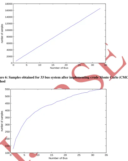
The samples obtained in crude Monte Carlo and importance sampling method for IEEE 33 bus system is shown
in figure 6 and 7 which indicates number of samples to be selected for individual bus. Table 2 indicates the
number of samples obtained in both the method. Lesser the sample lesser the variance thus computational time
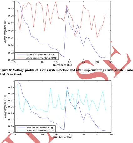
is reduced and increases the efficiency. Voltage profile of 33bus system before and after implementing crude
Monte Carlo (CMC) method and importance sampling method is shown in figure 8 and 9 respectively. This
shows less voltage fluctuation in the range 0.95-1.05 p.u.
Contingency analysis is performed for IEEE 33 bus system in which the load buses at 5,11,16,21,25,29 are
changed to generator bus and all the line resistance and reactance’s are changed to 100Ω. The performance
index for both active and reactive power is found, highest value of performance index is ranked first which
indicates severity. As per the results 24th bus is the most affected and 16th bus is less affected.
Figure 5: Voltage profile of 33 bus system before and after implementing DG
TABLE: 1
Simulation results of 33 bus system before and after placing DG
Loss in the initial bus system 208kW
Loss in the system after placing a DG 98.5kW
Loss reduction 109.5kW
Loss reduction [ %] 52.64%
0 5 10 15 20 25 30 35
0.92 0.93 0.94 0.95 0.96 0.97 0.98 0.99 1
Bus number
V
ol
ta
ge
in
p
.u
.
166 |
P a g e
Figure 6: Samples obtained for 33 bus system after implementing crude Monte Carlo (CMC)
method
Figure 7: Samples obtained for 33 bus system after implementing Importance sampling (IS)
method
TABLE: 2
Simulation result of 33 bus system after implementing the CMC and IS method
METHOD
Crude-Monte-Carlo
Importance sampling
Number-of-samples obtained for
IEEE-33-Bus system
16482 548
0 5 10 15 20 25 30 35
0 2000 4000 6000 8000 10000 12000 14000 16000 18000
Number of Bus
nu m be r of s am pl es
0 5 10 15 20 25 30 35
100 150 200 250 300 350 400 450 500 550
Number of Bus
167 |
P a g e
www.ijarse.com
Figure 8: Voltage profile of 33bus system before and after implementing crude Monte Carlo
(CMC) method.
Figure 9: Voltage profile of 33bus system before and after implementing Importance sampling
(IS) method.
VIII CONCLUSIONS
Voltage profile is improved by locating a DG using PSO which shows the loss reduction. Probability of failure
induced by changes in grid state is evaluated by Monte-Carlo simulation method. Analysis of
Crude-Monte-Carlo method and Importance sampling method is implemented to IEEE-33 bus system and results shows that
lesser the number of samples lesser the variance which improves the voltage stability.
0 5 10 15 20 25 30 35
0.92 0.93 0.94 0.95 0.96 0.97 0.98 0.99 1
Number of Bus
V ol ta ge m ag ni tu de in P .U before implementation after implementing CMC
0 5 10 15 20 25 30 35
0.92 0.93 0.94 0.95 0.96 0.97 0.98 0.99 1
Number of Bus
168 |
P a g e
REFERENCES
[1] IEEE/CIGRE joint task force on stability terms and definitions, “Definition and classification of power
system stability,” IEEE Trans. PowerSyst., vol. 19, no. 3, pp. 1387–1401, Aug. 2004.
[2] Q. Chen, C. Jiang, W. Qiu, and J. D. McCalley, “Probability models for estimating the probabilities of
cascading outages in high-voltage transmission network,” IEEE Trans. Power Syst., vol. 21, no. 3, pp. 1423–
1431, Aug. 2006.
[3] Q. Chen and J. D. McCalley, “Identifying high risk n-k contingencies for online security assessment,” IEEE
Trans. Power Syst., vol. 20, no. 2, pp. 823–834, May 2005.
[4] Y. Kataoka, “A probabilistic nodal loading model and worst case solutions for electric power system voltage
stability assessment”. IEEE Trans. Power Syst., vol. 18, no. 4, pp. 1507–1514, Nov. 2003.
[5] M. Perninge, V. Knazkins, M. Amelin, and L. Söder, “Risk estimation of critical time to voltage instability
induced by saddle-node bifurcation,” IEEE Trans. Power Syst., vol. 25, no. 3, pp. 1600–1610, Aug.2010.
[6] “Importance sampling of injected powers for electric power system security analysis”, IEEE transaction on
power system.
Vol-27, no-1, February 2012.
[7]C.W. Taylor, power system voltage stability. New York: McGraw-hill, 1993.
[8] N. Hampomchai, H. J. Pradlwarter and G. I. Schuëller, “Stochastic analysis of dynamical systems by
phase-space-controlled Monte Carlo simulation” Comput. Methods Appl. Mech. Eng., vol. 168, pp.273–283, 1999.
[9] Principles for Determining the Transfer Capacity in the Nordic Power Market, Nordel, 2008.
[10] S. Asmussen and P. W. Glynn, Stochastic Simulation. New York: Springer, 2007.
[11] Particle Swarm Optimization Based Method for Optimal Placement and Estimation of DG Capacity in
Distribution Networks, IJST, Volume 2 No.7, July 2012
[12] Jonathan Pengelly “Monte carlo methods” February 26, 2002.
[13] E. Afzalan1, M. A. Taghikhani2,*, M. Sedighizadeh1,2 “Optimal Placement and Sizing of DG in Radial