Indifferentiability of 10-Round Feistel Networks

(1)

Indifferentiability of 10-Round Feistel Networks

Yuanxi Dai and John Steinberger

Abstract. We prove that a (balanced) 10-round Feistel network is indifferentiable from a random permutation. In a previous seminal result, Holenstein et al. [17] had established indifferentiability of Feistel at 14 rounds. Our simulator achieves security O(q8_/₂n_{), runtime}_O₍_q4_{) and query complexity} O(q4_{), to be compared with security}_O₍_q10_/₂n_{), runtime} _O₍_q4_{) and query complexity} _O₍_q4_{) for the} 14-round simulator of Holenstein et al.

(2)

For many cryptographic protocols the only known analyses are in a so-calledideal primitive model. In such a model, a cryptographic component is replaced by an idealized information-theoretic counterpart (e.g., a random oracle takes the part of a hash function, or an ideal cipher substitutes for a concrete blockcipher such as AES) and security bounds are given as functions of the query complexity of an information-theoretic adversary with oracle access to the idealized primitive. Early uses of such ideal models include Winternitz [33], Fiat and Shamir [16] (see proof in [26]) and Bellare and Rogaway [2], with such analyses rapidly proliferating after the latter paper.

Given the popularity of such analyses a natural question that arises is to determine the relative “power” of different classes of primitives and, more precisely, whether one class of primitives can be used to “implement” another. E.g., is a random function always sufficient to implement an ideal cipher, in security games where oracle access to the ideal cipher/random function is granted to all parties? The challenge of such a question is partly definitional, since the different primitives have syntactically distinct interfaces. (Indeed, it seems that it was not immediately obvious to researchers that such a question made sense at all [7].)

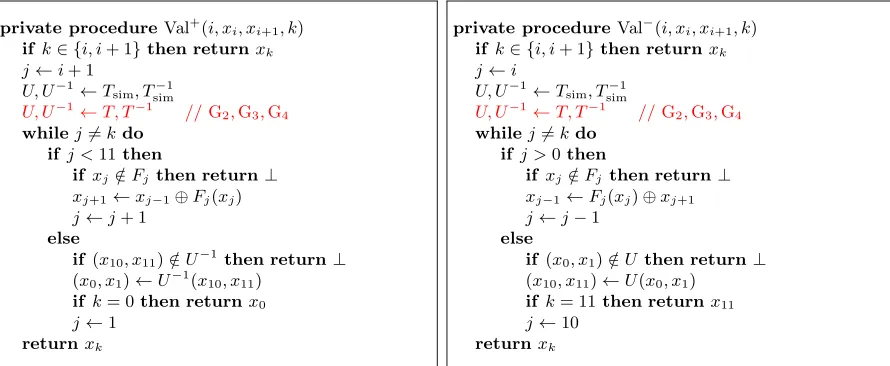
A sensible definitional framework, however, was proposed by Maurer et al.[21], who introduce a simulation-based notion ofindifferentiability. This framework allows to meaningfully discuss the instantiation of one ideal primitive by a syntactically different primitive, and to compose such results. (Similar simulation-based definitions appear in [4, 5, 24, 25].) Coron et al. [7] are early adopters of the framework, and give additional insights.

(3)

π

_A

P

C

π

_A

S

Z

π

_A

′

Z

Fig. 1.The cliff notes of indifferentiability, after [7]: (left) adversaryAinteracts in a game with protocolπin whichπ calls a constructionC that calls an ideal primitivePand in whichAcallsPdirectly; (middle) by indifferentiability, the pair (CP

,P) can be replaced with the pair (Z, SZ

), whereZis an ideal primitive matchingC’s syntax, without significantly affecting A’s probability of success; (right) folding S into A gives a new adversary A′

for a modified security game in which the “real world” construction CP _{has been replaced by the “ideal world” functionality}

Z. Hence, a lack of attacks in the ideal world implies a lack of attacks in the real world.

For example, Coron et al. [7] already showed that random oracles can be instantiated from ideal ciphers in this sense, using constructions that are similar to the Merkle-D˚amgard iteration of a blockcipher in Davies-Meyer mode. Naturally, one would also like to consider the reverse direction, i.e., the implementation of an ideal cipher from a random function. This direction has revealed itself to be more challenging.

The natural candidate for a construction (and echoing the construction of pseudorandom per-mutations from pseudorandom functions by Luby and Rackoff [20]) is a (balanced, keyed) Feis-tel network. (Since all our Feistel networks are going to be balanced, we will subsequently drop this qualifier.) An unkeyed Feistel network is shown in Fig. 2. If each wire carries n bits, then the network implements a 2n-bit to 2n-bit permutation for any choice of the round functions

Fi : {0,1}n → {0,1}n. “Keyeing” the network means extending the domain of each Fi from n

bits to n+κ bits, where κ is the length of the key; if the Fi’s are random, one then recovers 2κ

independent (though not necessarily “random”) permutations from 2nto 2nbits, i.e., one recovers a blockcipher of key lengthκand of word length 2nin which each key behaves independently from every other key.

Due to the trick of domain extension just mentioned, it suffices1 _{to show that an unkeyed} _r -round Feistel network with random -round functions is indifferentiable from a random permutation in order to implement a blockcipher from a random function. (Ther independent round functions fromnbits tonbits can be implemented from a single random function with slightly larger domain.) Consequently, much work has focused on the previous question.

The first paper directly in this line [9] shows that an r-round Feistel network cannot be in-differentiable from a random permutation for r ≤ 5. The same paper also gives a proof that indifferentiability is achieved at r = 6. The second result, however, was found to have a serious

1_{A fact that authors tend to gloss over, however, is that there is an additional security loss—specifically, a factor}_q whereqis the number of distinguisher queries—in going from the unkeyed to the keyed setting. Moreover this loss seems intrinsic: consider the case of a family of functionsF1, . . . , Fr:{0,1}n+κ→ {0,1}n for which there exists a (random) subsetT ⊆ {0,1}κ_{of size 2}κ_/_{1000 such that for all}_k_∈_T_{, the functions}_F

1(·, k), . . . , Fr(·, k) :{0,1}n→ {0,1}n _{are identically zero, while for all} _{k /}

(4)

flaw by Holenstein et al.[17], and who could indeed not repair the simulator at six rounds; instead, Holenstein et al.could only show that a 14-round Feistel network is indifferentiable from a random permutation. Holenstein et al. also found a flaw in the proof of indifferentiability for a 10-round simulator of Seurin [29] (a simplified alternative to the 6-round simulator of [9]) and Seurin himself subsequently found a clever attack against his own simulator, thus showing that the proof could not be patched [30]. On the other hand, it should be noted that the 14-round simulator of Holen-stein et al. follows design principles that are very similar to Seurin’s 10-round simulator; indeed, the 14-round simulator essentially consists of Seurin’s 10-round simulator with four extra “buffer rounds” flanking the simulator’s two “adapt zones”.

Our purpose in this work is to recommence the “downward journey” in the number of rounds of Feistel that are known to be sufficient to achieve indifferentiability from a random permutation. Specifically, we show that 10 rounds suffice, while achieving basically the same security and query complexity as the 14-round simulator of Holenstein et al.2 Our simulator is also closely based on Seurin’s 10-round simulator, with the minor (but technically significant) difference that our simulator completes paths in LIFO fashion rather than in FIFO fashion: the last path detected is given priority for completion over paths that are already under completion. In particular, this change happens to circumvent Seurin’s 10-round attack.

We note that the change from FIFO to LIFO path completion has deep structural repercussions for our proof, which ends up looking quite different from the indifferentiability proof of Holenstein et al.[17]. In our case, in particular, the concurrent completion of several paths unfolds in a highly structured manner that makes it easy to maintain a complete picture of the state of partially completed paths at any point in time. The soundness of our simulator ends up being quite a bit more intuitive than the simulator of [17].

Concurrent Work. Katz et al. [18] have also announced a 10-round indifferentiability result; the two teams have been in communication in order to coordinate the release of results, but as of going to print neither team has seen the technical details of the other’s work.

We also expect the techniques of this paper to yield further improvements in security and round complexity for Feistel simulators. This is ongoing work.

Other Related Work.Even before [9] Dodis and Puniya [10] investigated the indifferentiability of Feistel networks in the so-calledhonest-but-curiousmodel, which is incomparable to the standard notion of indifferentiability. They found that in this case, a super-logarithmic number of rounds is sufficient to achieve indifferentiability. Moreover, [9] later showed that super-logarithmically many rounds are also necessary.

Besides Feistel networks, the indifferentiability of many other types of constructions (and par-ticularly hash functions and compression functions) have been investigated. More specifically on the blockcipher side, however, [1] and [19] investigate the indifferentiability of key-alternating ciphers (with and without an idealized key scheduler, respectively). In a recent eprint note, Dodis et al.[11] investigate the indifferentiability of substitution-permutation networks, treating theS-boxes as in-dependent idealized permutations; as we will mention later, our simulator is also partly inspired by theirs.

It should be noted that indifferentiability does not apply to a cryptographic game for which the adversary is stipulated to come from a special class that does not contain the computational class

(5)

to which the simulator belongs (the latter class being typically “probabilistic polynomial-time”). This limitation was first noted by Ristenpart et al. [27], who moreover give a interesting example where indifferentiability serves no use.

Finally, Feistel networks have been the subject of a very large body of work in the secret-key (or “indistinguishability”) setting, such as in [20, 22, 23, 28] and the references therein.

Paper Organization. In Section 2 we give the few definitions necessary concerning Feistel net-works and indifferentiability, and we also state our main result.

In Section 3 we give an intuitive overview of our simulator, focusing on high-level design prin-ciples. A more technical description of the simulator (starting from scratch, and also establishing some of the terminology used in the proof) is given in Section 4. Section 5 contains the proof itself, starting with a short overview of the proof.

2 Definitions and Main Result

Feistel Networks.Letr≥0 and letF1, . . . , Fr :{0,1}n→ {0,1}n. Given valuesx0, x1 ∈ {0,1}n we define values x2, . . . , xr+1 by

xi+1=Fi(xi)⊕xi−1 for 1≤i≤r. It is easy to see that the application

(x0, x1)→(xr, xr+1)

is a permutation, since xi−1 can be computed from xi and xi+1 for 1≤i≤r−1. We denote the resulting permutation of {0,1}2n _as

Ψ[F1, . . . , Fr].

We say that Ψ is anr-round Feistel network and that Fi is thei-th round function.

In this paper, whenever a permutation is given as an oracle, our meaning is that both forward and inverse queries can be made to the permutation. This implies in particular to Feistel networks.

Indifferentiability.Aconstruction is a stateless deterministic algorithm that evaluates by mak-ing calls to an external set of primitives. The latter are functions that conform to a syntax that is specified by the construction. For example, Ψ[F1, . . . , Fr] can be seen as a construction with

primitivesF1, . . . , Fr. In the general case we notate a constructionC with oracle access to a set of

primitivesP asCP.

A primitive isideal if it is drawn uniformly at random from the set of all functions meeting the specified syntax. Arandom function F :{0,1}n_{→ {0}_,_1}n _{is a particular case of an ideal primitive.}

Such a function is drawn uniformly at random from the set of all functions of domain {0,1}n _and

of range{0,1}n_.

Asimulator is a stateful randomized algorithm that receives and answer queries, possibly being given oracles of its own. We assume that a simulator is initialized to some default state (which constitutes part of the simulator’s description) at the start of each experiment. A simulatorS with oracle(s)Z is notated as SZ_.

(6)

distinguisher can “know by heart” the (adaptive) sequence of questions that will maximize its dis-tinguishing advantage. In particular, one may assume without loss of generality that a distinguisher is deterministic.

Indifferentability seeks to determine when a constructionCP_{, where}_P_{is a set of ideal primitives,} is “as good as” an ideal primitive Z that has the same syntax (interface) as CP. In brief, there must exist a simulator S such that having oracle access to the pair (CP_,_P_{) (often referred to as} the “real world”) is indistinguishable from the pair (Z, SZ_{) (often referred to as the “simulated} world”).

In more detail we refer to the following definition, which is due to Maurer et al.[21].

Definition 1. A constructionCwith access to a set of ideal primitivesP is(tS, qS, ε)-indifferentiable from an ideal primitive Z if there exists a simulator S =S(q) such that

PrhDCP,P = 1i−PrhDZ,SZ = 1i≤ε

for every distinguisher D making at most q queries in total, and such that S runs in total time tS and makes at most qS queries toZ. Here tS, qS and εare functions of q, and the probabilities are taken over the randomness in P, Z, S and (if any) inD.

As indicated, we allow S to depend onq.3 _{The notation}

DCP,P

indicates that Dhas oracle access to CP _{as well as to each of the primitives in the set} _{P. We also} note that the oracle

SZ

offers one interface for D to query for each of the primitives in P; however the simulator S is “monolithic” and treats each of these queries with knowledge of the others.

Thus,S’s job is to makeZ look like CP _{by inventing appropriate answers for}_D_{’s queries to the} primitives in P. In order to do this, S requires oracle access to Z. On the other hand, S doesn’t know which queries Dis making toZ.

Informally,CPisindifferentiablefromZif it is (tS, qS, ε)-indifferentiable for “reasonable” values

of tS, qS and for ε negligibly small in the security parameter n. The value qS in Definition 1 is

called the query complexity of the simulator.

In our setting C will be the 10-round Feistel network and P will be the set {F1, . . . , F10} of round functions, with each round function being an independent random function. Consequently, Z (matchingCP_{’s syntax) will be a random permutation from}_{0_,_1}2n _to _{0_,_1}2n_{, queriable (like} CP) in both directions; this random permutation is notatedP in the body of the proof.

Main Result.The following theorem is our main result. In this theorem, Ψ plays the role of the construction C, while{F1, . . . , F10} (where each Fi is an independent random function) plays the

role of P, the set of ideal primitives called byC.

(7)

Theorem 1. The Feistel networkΨ[F1, . . . , F10]is(tS, qS, ε)-indifferentiable from a random 2n-bit to 2n-bit permutation with tS =O(q4), qS = 16q4 and ε= 6023424q8/2n. Moreover, these bounds hold even if the distinguisher is allowed to make q queries to each of its 11 (= 10 + 1) oracles.

The simulator that we use to establish Theorem 1 is described in the two next sections. The three seperate bounds that make up Theorem 1 (for tS,qS and ε) are found in Theorems 34, 31 and 84

of sections 5.1, 5.1 and 5.7 respectively.

Miscellaneous Notations. Our pseudocode uses standard conventions from object-oriented programming, including consutrctors and dot notation ‘.’ for field accesses. (Our objects, however, have no methods save constructors.)

We write [k] for the set {1, . . . , k}, k∈N_.

The symbol ⊥denotes an uninitialized or null value (and can be taken to be synonymous with a programming language’s null value, though we reserve the latter for uninitialized object fields). If T is a table, moreover, we write x ∈T to mean that T(x)6=⊥. Correspondingly, x /∈T means

T(x) =⊥.

3 High-Level Simulator Overview

In this section we try to convey the “design philosophy” of our simulator which, like [17], is a modification of a 10-round simulator by Seurin [29].

Round Function Tables. We recall that the simulator is responsible for 10 interfaces, i.e., one for each of the rounds functions. These interfaces are available to the adversary through a single function, named

F

in our pseudocode (see Fig. 3 and onwards), and which takes two inputs: an integeri∈[10] and an input x∈ {0,1}n_.

Correspondingly to these 10 interfaces, the simulator maintains 10 tables, notated F1, . . . , F10, whose fields are initialized to ⊥: initially,Fi(x) =⊥for allx∈ {0,1}n, alli∈[10]. (Hence we note

thatFi is no longer the name of a round function, but the name of a table, which should not cause

confusion. The i-th round function is now F(i,·).) The table Fi encodes “what the simulator has

decided so far” about the i-th round function. For instance, ifFi(x) =y 6=⊥, then any subsequent

distinguisher query of the form F(i, x) will returny. Moreover, entries in the tablesF1, . . . , F10are never overwritten once they have been set to non-⊥ values.

The 2n-bit Random Permutation.Additionally, the distinguisher and the simulator both have oracle access to a random permutation on 2nbits, notated

P

in our pseudocode (see Fig. 6), and which plays the role of the ideal primitive Z in Definition 1. Thus P accepts an input of the form (x0, x1)∈ {0,1}n×{0,1}nand produces an output (x10, x11)∈ {0,1}n_{× {0}_,_1}n_{. P’s inverse P}−1 _{is also available as an oracle to both the distinguisher and the} simulator.

(8)

could choose random valuesx0, x1 ∈ {0,1}n, construct the values x2, . . . , x11 by setting

xi+1←xi−1⊕F(i, xi)

fori= 1, . . . ,10, and finally check if (x10, x11) = P(x0, x1). (In the real world, this will always be the case; if the simulator is doing its job, it should also be the case in the simulated world.) In this case we also say that the values

x1, . . . , x10

queried by the distinguisher form a completed path. (The definition of a “completed path” will be made much more precise in the next section. The terminology that we use in this section is hand-wavy through and through.)

Moreover, the distinguisher need not complete paths in left-to-right fashion: it might choose, e.g., valuesx4 andx5at random, and build a completed path outwards from those positions (“going left” for x3,x2 and x1, “going right” for x6, . . . , x10). Or it might, say, choose random values x0,

x1, make the query

(x10, x11)←P(x0, x1)

and then complete from both ends at once (making some queries on the left starting from x0,x1, and some queries on the right starting fromx10,x11). Other possibilities can be imagined as well. Moreover, the distinguisher may reuse the same queries for several different paths.

To summarize, and for the purpose of intuition, one can picture the distinguisher as trying to complete all sorts of paths in a convoluted fashion in order to confuse and/or “trap” the simulator in a contradiction.

The Simulator’s Dilemma. Clearly a simulator must to some extent detect which chains a distinguisher is trying to complete, and “adapt” the values along chains such as to be compatible with P. Concerning the latter, one can observe that a pair of missing consecutive queries is sufficient to adapt the two ends of a chain to one another; thus if, say,

x1, x2, x5, x6, x7, x8, x9, x10

are values such that

Fi(xi)6=⊥

for all i∈ {1,2,5,6,7,8,9,10}, and such that

xi+1=xi−1⊕Fi(xi)

fori∈ {6,7,8,9}, and such that

P(x0, x1) = (x10, x11) wherex0:=F1(x1)⊕x2,x11:=x9⊕F10(x10), and such that

F3(x3) =F4(x4) =⊥

wherex3:=x1⊕F2(x2),x4:=F5(x5)⊕x6, then by making the assignments

F3(x3)←x2⊕x4 (1)

(9)

the simulator turnsx1, . . . , x10 into a completed path that is compatible with P. In such a case, we say that the simulatoradapts a path. The values F3(x3) and F4(x4) are also said to beadapted.

In general, however, if the simulator always waits until the last minute (e.g., until only two adjacent undefined queries are left) before adapting a path, it can become caught in an over-constrained situation whereby several different paths request different adapted values at the same position. Hence, it is usual for simulators to give themselves a “safety margin” and to pre-emptively complete paths some time in advance. When pre-emptively completing a path, typical simulators sample all but two values along the path randomly, while “adapting” the last two values as above. Here it should be emphasized that our simulator, like previous simulators [9, 17, 29], makes no distinction between a non-null valueFi(xi) that is non-null because the distinguisher has made the

query F(i, xi) or that is non-null because the simulator has set the valueFi(xi) during a pre-emptive

path completion. (Such a distinction seems tricky to leverage, particularly since the distinguisher can know a valueFi(xi) without making the query F(i, xi), simply by knowing adjacent values and

by knowing how the simulator operates.) Moreover, the simulator routinely calls its own interface F(·,·)

during the process of path completion, and it should be noted that our simulator, again like previous simulators, makes no difference between distinguisher calls to F and its own calls to F.

One of the basic dilemmas, then, is to decide at which point it is worth it to complete a path; if the simulator waits too long, it is prone to finding itself in an over-constrained situation; if it is too trigger-happy, on the other hand, it runs the danger of creating out-of-control chain reactions of path completions, whereby the process of completing a path sets off another path, and so on. We refer to the latter problem (that is, avoiding out-of-control chain reactions) as the problem of

simulator termination.

Seurin’s 10-Round Simulator.Our starting point is a 10-round simulator of Seurin [29], which nicely handles the problem of simulator termination.

F1

x0 x1

F2 x2

F3 x3

F4 x4

F5 x5

F6 x6

F7 x7

F8 x8

F9 x9

F10 x10

x11 detect

adapt adapt

detect detect

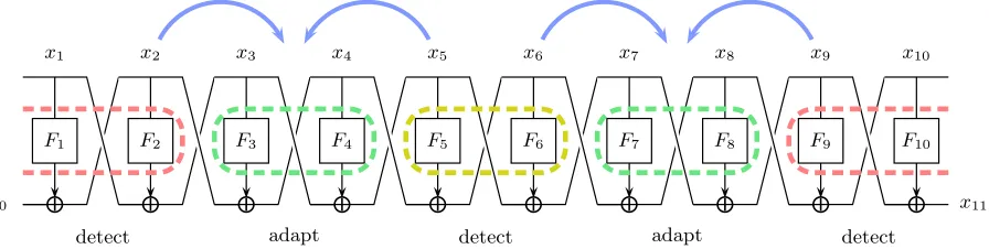
Fig. 2.A sketch of our 10-round simulator (and also Seurin’s). Rounds 5 and 6 form one detect zone; rounds 1, 2, 9 and 10 form another detect zone; rounds 3 and 4 constitute the left adapt zone, 7 and 8 constitute the right adapt zone; blue arrows point from the position where a path is detected to the adapt zone for that path.

In a nutshell, Seurin’s simulator completes a path for every pair of values (x5, x6) such that

F5(x5) andF6(x6) are defined, as well as for every 4-tuple of values

(10)

such that

F1(x1), F2(x2), F9(x9), F10(x10) are all defined, and such that

P(x0, x1) = (x10, x11) wherex0:=F1(x1)⊕x2,x11:=x9⊕F10(x10).

Paths are adapted either at positions 3, 4 or else at positions 7, 8. (See Fig.2.)

In a little more detail, a function call F(5, x5) for whichF5(x5) =⊥triggers a path completion for every valuex6such thatF6(x6)6=⊥; such paths are adapted at positions 3 and 4. Symmetrically, a function call F(6, x6) for whichF6(x6) =⊥triggers a path completion for every valuex5such that

F5(x5)6=⊥; such paths are adapted at positions 7 and 8. For the second type of path completion, a call F(2, x2) such thatF2(x2) =⊥triggers a path completion for every tuple of valuesx1,x9,x10 such that F1(x1), F9(x9) and F10(x10) are defined, and such that the constraints listed above are satisfied (verifying these constraints thus requires a call to P or P−1_{); such paths are adapted at} positions 3, 4. Paths that are symmetrically triggered by a query F(9, x9) are adapted at positions 7, 8. Function calls to F(2,·), F(5,·), F(6,·) and F(9,·) are the only ones to trigger path completions. (Indeed, one can easily convince oneself that sampling a new value F1(x1) or F10(x10) can only trigger the second type of path completion with negligibly low probability; hence, this possibility is entirely ignored by the simulator.) To summarize, in all cases the completed path is adapted at positions that are immediately next to the query that triggers the path completion.

To more precisely visualize the process of path completion, imagine that a query F(2, x2)

has just triggered the second type of path completion, for some corresponding values x1, x9 and

x10; then Seurin’s simulator (which would immediately lazy sample the value F2(x2) even before checking if this query triggers any path completions) would (a) make the queries

F(8, x8), . . . ,F(6, x6),F(5, x5)

to itself in that order, wherexi−1 :=Fi(xi)⊕xi+1= F(i, xi)⊕xi+1 fori= 9, . . . ,6, and (b) adapt the values F3(x3), F4(x4) as in (1), (2) where x3 := x1⊕F2(x2), x4 := F5(x5)⊕x6. In general, some subset of the table entries

F8(x8), . . . , F5(x5)

(and more exactly, a prefix of this sequence) may be defined even before the queries F(8, x8),

. . . ,F(5, x5) are made. The crucial fact to argue, however, is thatF3(x3) =F4(x4) =⊥right before these table entries are adapted. Other types of path completions are carried out analogously; for example, if F6(x6) =⊥when the query

F(6, x6)

is made, then this query F(6, x6) will trigger another path completion for every value x∗5 such that

F5(x∗5) 6=⊥at the moment when the query F(6, x6) occurs; and such a path completion proceeds by making (possibly redundant) queries

F(4, x∗₄), . . . ,F(1, x∗₁),F(10, x∗₁₀),F(9, x∗₉)

(11)

The crucial fact to argue is (again) that F7(x∗7) =F8(x∗8) =⊥ when it comes time to adapt these table values, wherex∗₈ :=F10(x∗₁₀)⊕x₁₁∗ ,x∗₇ :=x∗₅⊕F6(x6).

In Seurin’s simulator, moreover, paths are completed on a first-come-first-serve (or FIFO4) basis: while paths are “detected” immediately when the query that triggers the path completion is made, this information is shelved for later, and the actual path completion only occurs after all previously detected paths have been completed. The imbroglio of semi-completed paths is rather difficult to keep track of, however, and indeed Seurin’s simulator was later found to suffer from a real “bug” related to the simultaneous completion of multiple paths [17, 30].

Changes to Seurin’s Simulator.For the following discussion, we will say that the table entries

F2(x2), F5(x5) constitute the endpoints of a completed path x1, . . . , x10 that is adapted at posi-tions 3, 4; likewise, the table entries F6(x6), F9(x9) constitute the endpoints of a completed path

x1, . . . , x10 that is adapted at positions 7, 8. Hence, the endpoints are the two table entries that “flank” the adapted entries. Succinctly, our simulator’s philosophy is to not sample the endpoints of a completed path until right before the path is about to be adapted or (even more succinctly!)

to sample randomness at the moment it is needed. This essentially results in two main differences for our simulator, which are (i) changing the order in which paths are completed and (ii) doing “batch adaptations” of paths, i.e., adapting several paths at once, for paths that happen to share endpoints.

To illustrate the first point, return to the above example of a query F(2, x2)

that triggers a path completion of the second type with respect to some values x1,x9,x10. Then by definition

F2(x2) =⊥

at the moment when the call F(2, x2) is made. Instead of immediately lazy samplingF2(x2), as in the original simulator, we will keep this value “pending” (the technical term that we use in the proof is “pending query”) until the path is ready to be adapted. (Technically, “ready to be adapted” means, for a path that is adapted in positions 3 and 4, that both of the valuesx2 andx5 are known; for a path adapted in positions 7 and 8, that both of the values x6,x9 are known.) Moreover, and keeping the notations from the previous example, note that the query

F(6, x6)

will itself become a “pending query” at position 6 as long as there is at least one valuex∗

5 such that

F5(x∗5) 6=⊥, since in such a case x6 is the endpoint of a path-to-be-completed (namely, the path which we notated as x∗₁, . . . , x∗₅, x6, x∗7, . . . , x∗10 above), and, according to our policy, this endpoint must be kept unsampled until the corresponding path is ready to be adapted. In particular, the value x5 =F6(x6)⊕x7 from the “original” path cannot be computed until the “secondary” path containingx∗₅ andx6 has been completed (or even more: untilall secondary paths triggered by the query F(6, x6) have been completed). In other words, the query F(6, x6) “holds up” the completion of the first path. In practical terms, paths that are detected during the completion of another path take precedence over the original path, so that path completion becomes a LIFO process. (Of course, one must show that cyclic dependencies don’t arise except with negligible probability; this is done in the proof.)

(12)

Next, to describe the “batch adaptation” of paths, say (for now) that a table entry

Fj(xj)

for j ∈ {2,5,6,9} is a pending query if Fj(xj) = ⊥ and the call F(j, xj) has been made and has

triggered at least one path completion. Moreover, say that two pending queries arelinked if they are the two endpoints of the same yet-to-be-completed path (in which case we say that the path is “ready to be adapted”, as described above). Moreover a pending query Fj(xj) is stable if it does

not currently5 _{trigger a path completion. (Paths that are already ready to be adapted do not count} as potential triggers.)

Pending queries can be represented by a graph, with a node for each pending query and an edge for each linked pair of pending queries. Thus, each edge corresponds to a path that is ready to be adapted and vice-versa. If we say that a vertex corresponding to pending queryFj(xj) is in

“shorej”, then edges only exist between vertices in shores 2 and 5 on the one hand and between vertices in shores 6 and 9 on the other hand. Moreover, one can show that, with high probability, each connected component is a tree. We say that a tree is stable if all its nodes are stable.

To picture the evolution of this graph over time, when the distinguisher initially makes a query F(j, xj) the graph is empty, because there are no pending queries. If j /∈ {2,5,6,9} then the

simulator lazy samples the value Fj(xj) if does not already exist, and simply returns Fj(xj) to

the distinguisher. Otherwise, right after the query is made, the graph contains at most one node, namely the pending query Fj(xj), which has triggered one or more path completions if the graph

is nonempty. From there, the simulator “grows”6 _{a tree containing this node; the tree spans shores} 2, 5 if j ∈ {2,5} and spans shores 6, 9 if j ∈ {6,9}. At any point the growth of a tree spanning shores 2, 5 may be interrupted by the apparition of a tree spanning shores 6 and 9, and vice-versa. Hence a “stack of trees” (alternating between trees of shore 2, 5 and trees of shore 6, 9) is created, where only the last (topmost) tree on the stack is being grown at any time. The topmost tree is also the only tree that potentially becomesstable, with trees lower down in the stack being unstable by virtue of still being under construction. The proof also shows that new trees do not “collide” with older trees as they grow.

If and when the topmost tree on the stack becomes stable, the simulator adapts the paths corresponding to edges in this tree all at once. This happens in two stages: first the simulator lazy samples the values of all pending queries (a.k.a.nodes) in the tree; then, for each path (a.k.a.edge) the simulator adapts last two queries on the path as in (1), (2) (or using the analogous equations for F7, F8). This two-step process is what we refer to as “batch adaptation”. After the tree has been adapted, it disappears and the simulator resumes work on the next topmost tree in the stack.

Structural vs. Conceptual Changes. Of the two main changes to Seurin’s simulator just described it should be noted that the first (i.e., LIFO path completion) is crucial to the correctness of our simulator, whereas the second (i.e., batch adaptations) is only a conceptual convenience, not necessary for correctness. Indeed, one way or another every non-null value

Fj(xj)

5_{Here “currently” emphasizes that the query does not trigger a path completion}_{with respect to the current contents} of the tables{Fi}10

i=1as opposed to with respect to the “old” contents of the same tables at the point in time when the query F(j, xj) was originally made.

(13)

forj /∈ {3,4,7,8} ends up being randomly and independently sampled in our simulator, as well as in Seurin’s; so one might as well load a random value into Fj(xj) as soon as the query F(j, xj) is

made, as in Seurin’s original simulator. This approach ends up being correct, but is conceptually less convenient, since the “freshness” of the random value Fj(xj) is harder to argue when that

randomness is needed (e.g., to argue that adapted queries do not collide, etc). In fact, our simulator is an interesting case where the search for a syntactically convenient usage of randomness naturally leads to structural changes that turn out to be critical for correctness.

We also point out that the idea of batch adaptations already appears explicitly in the simulator of [11], and which indeed formed part of the inspiration for our own work. In [11], however, batch adaptations are purely made for conceptual convenience.

Finally, readers seeking even more concrete insights can consult Seurin’s attack against his own 10-round simulator [30] and check this attack fails when the simulator is switched to LIFO path completion.

The Termination Argument. For completeness, we also briefly reproduce Seurin’s (by now classic) termination argument.

The basic idea is that each path of the second type—that is, paths detected at position 2 or 9—is associated to a previously existing P-query, and one can show that this P-query is, with high probability, first made by the distinguisher. Since the distinguisher only has q queries total, this already implies that the number of path completions of the second type is at most q.

Secondly, path completions of the first type do not actually add any entries to either of the tables F5 or F6. Hence, only two mechanisms add entries to the tables F5 and F6: queries directly made by the distinguisher and path completions of the second type. Each of these accounts for at mostq table entries, so that the tablesF5,F6 do not exceed size 2q. This implies that the number of path completions of the first type is at most (2q)2 _{and the total number of all path completions} is at most 4q2+q.

4 Technical Simulator Overview and Pseudocode Description

In this section we “reboot” the simulator description, with a view to the proof of Theorem 1. A number of terms introduced informally in Section 3 are given precise definitions here. As already admonished, indeed, the provisory definitions and terminology of Section 3 should not be taken seriously as far as the main proof is concerned.

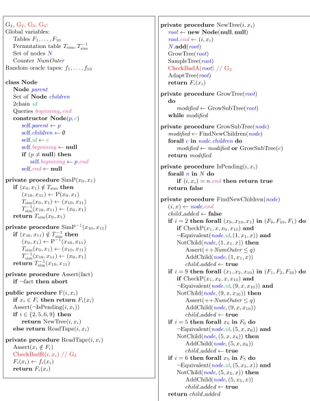
The pseudocode describing our simulator is given in Figs. 3–5, and more specifically by the pseudocode for game G1, which is the simulated world. In Fig. 3, in particular, one finds the function F (to be called with an argument (i, x) ∈ [10]× {0,1}n_{), which is the simulator’s only}

interface to the distinguisher. The random permutation P and its inverse P−1—which are the other interfaces available to the distinguisher—can be found on the left-hand side of Fig.6, which is also part of game G1.

Our pseudocode uses explicit random tapes, similarly to [17]. On the one hand there are tapes

f1, ..., f10 where fi is a table of 2n randomn-bit values for each 1≤i≤10, i.e.,fi(x) is a uniform

independent randomn-bit value for each 1≤i≤10 and eachx∈ {0,1}n_{. Moreover there is a tape} p:{0,1}2n_{→ {0}_,_1}2n _{that implements a random permutation from 2}_n_{bits to 2}_n_{bits. The inverse}

of pis accessible viap−1_{. The only procedures to access}_p _and _p−1 _{are P and P}−1_.

As described in the previous section, the simulator maitains a table Fi :{0,1}n → {0,1}n for

(14)

simulator fills the tablesFi progressively, and never overwrites a value Fi(x) such thatFi(x)6=⊥.

If a call to F(i, x) occurs andFi(x)6=⊥, the call simply returnsFi(x).

The permutation oracle P/P−1 _{also maintains a pair of private tables} _{T /T}−1 _{that encode a} subset of the random tapesp/p−1. We refer to Fig.6 for details (briefly, however, the tablesT /T−1

remember the values on which P/P−1 have already been called). These tables serve no tangible purpose in G1, where P/P−1 implement black-box two-way access to a random permutation, but they serve a role subsequent games, and they appear in some of the definitions below.

If a call F(i, x) occurs and Fi(x) =⊥ andi /∈ {2,5,6,9}, the simulator sets Fi(x) ←fi(x) and

returns this value. Otherwise, ifi∈ {2,5,6,9} and ifFi(x) =⊥, the pair (i, x) becomes a “pending

query”, as formally defined below.

In certain situations, and following [1], our simulator explicitly aborts (‘abort’). In such cases the distinguisher is notified of the abort and the game ends.

In order to describe the operation of the simulator in further detail we introduce some more terminology.

A query cycle is the portion of simulator execution from the moment the distinguisher makes a query to F(·,·) until the moment the simulator either returns a value to the distinguisher or aborts. A query cycle isnon-aborted if the simulator does not abort during that query cycle.

A query is a pair (i, x)∈[10]× {0,1}n_{. The value}_i_{is the} _position _{of the query.}

A query (i, x) is defined if Fi(x) 6= ⊥. Like many other predicates defined below, this is a

time-dependent property.

Our simulator’s central data type is a Node. (See Fig. 3.) Nodes are arranged into trees. A node n is the root of its tree if and only if n.parent=null. Node b is the child of nodea if and only if b∈a.children and if and only ifb.parent=a. Each tree has a root.

Typically, several disjoint trees will coexist during a given query cycle. Distinct trees are never brought to merge. Moreover, new tree nodes are only added beneath existing nodes, as opposed to above the root. (Thus the first node of a tree to be created is the root, and this node remains the root as long as the tree exists.) Nodes are never deleted from trees, either. However, a tree is “lost” once the last reference to the root pops off the execution stack, at which point we say that the tree and its nodes have beendiscarded. Instead of garbage collecting discarded nodes, however, we assume that such nodes remain in memory somewhere, for convenience of description within the proof. Thus, once a node is created it is not destroyed, and we may refer to the node and its fields even while the node has no more purpose for the simulator.

Besides the parent/child fields, a node contains abeginning and an end, that are both queries, possiblynull, i.e., beginning, end ∈ {[10]× {0,1}n_,_null_{}. In fact}

beginning, end ∈ {{2,5,6,9} × {0,1}n,null} more precisely.

The beginning and end fields are never overwritten after they are set to non-null values. A node n such that n.end 6= null is said to be ready, and a node cannot have children unless it is ready. The root n of a tree has n.beginning = null, while a non-root node n has n.beginning =

n.parent.end (which is non-null since the parent is ready). Hence n is the root of its tree if and only if n.beginning=null.

A query (i, x) is pending if and only ifFi(x) =⊥and there exists a node nsuch that n.end=

(15)

Fi(x) = ⊥ and such thati∈ {2,5,6,9}, a call NewTree(i, x) occurs that results a new tree being

created, with a root nsuch thatn.end= (i, x), so that (i, x) becomes a pending query.

Intuitively, a query (i, x) is pending ifFi(x) =⊥but the simulator has already decided to assign

a value toFi(x) during that query cycle. A query can only be pending for i= 2, 5, 6 or 9, since a

pending query is the end field of some node (see the remark above about the limited positions at which beginning and end appear).

The following additional useful facts about trees will be seen in the proof: 1. We have

a.end6=b.end

for all nodesa6=b, presuminga.end, b.end6=null, and regardless of whetheraandb are in the same tree or not. (Thus all query fields in all trees are distinct, modulo the fact that a child’s

beginning is the same as its parent’s end.)

2. If n.beginning= (i, xi)6=null,n.end= (j, xj)6=nullthen

{i, j} ∈ {{2,5},{6,9}}.

3. Each tree has at most one non-ready node, i.e., at most one node n with n.end =null. This node is necessarily a leaf, and, if it exists, is called the non-ready leaf of the tree.

4. GrowTree(root) is only called once per root root, as syntactically obvious from the code. While this call has not yet returned, moreover, we haveFi(x) =⊥for all (i, x) such thatn.end= (i, x)

for some node n of the tree. (In other words, a pending query remains pending as long as the node to which it is associated belongs to a tree which has not finished growing.)

The origin of a node n is the position ofn.beginning, ifn.beginning6=null. Theterminal of a nodenis the position ofn.end, ifn.end6=null. (Thus, as per the second bullet above, if the origin is 2 the terminal is 5 and vice-versa, whereas if the origin is 6 the terminal is 9 and vice-versa.)

A 2chain is a triple of the form (i, xi, xi+1)∈ {0,1, . . . ,10} × {0,1}n× {0,1}n. The position of

the 2chain isi.

Each node has a 2chain field called id, which is non-null if and only if the node isn’t the root of its tree. The position of id isi−1 if the node has origin i∈ {2,6}; the position of id is iif the node has origini∈ {5,9}.

Intuitively, each node that is ready is associated to a path from its origin to its terminal, and theid contains the first two queries on the path; indeed the first two queries are enough to uniquely determine the path (provided the relevant table values are present).

The simulator also maintains a global list N of nodes that are ready. This list is maintained for the convenience of the procedure IsPending, which would otherwise require searching through all trees that have not yet been discarded (and, in particular, maintaining a set of pointers to the roots of such trees).

Recursive call structure.Trees are grown according to a somewhat complex recursive mech-anism. Here is the overall recursive structure of the stack:

– F calls NewTree (at most one call to NewTree per call to F)

(16)

– GrowSubTree calls FindNewChildren (one or more times) and also calls GrowSubTree (zero or more times)

– FindNewChildren calls AddChild (zero or more times)

– AddChild calls MakeNodeReady (one call to MakeNodeReady per call to AddChild) – MakeNodeReady calls Prev or Next (zero or more times)

– Prev and Next call F (zero or once)

We observe that new trees are only created by calls to F. Moreover, a node n is not ready (i.e., n.end = null) when MakeNodeReady(n) is called, and can be seen by direct inspection of the pseudocode, and n is ready (i.e., n.end 6= null) when MakeNodeReady(n) returns, whence the name of the procedure. Since MakeNodeReady calls Prev and Next (which themselves call F), entire trees might be created and discarded while making a node ready.

Tree Growth Mechanism and Path Detection. Recall that every pending query (i, x) is uniquely associated to some node n (in some tree) such that n.end= (i, x). Every pending query is susceptible of triggering zero or more path completions, each of which incurs the creation of a new node that will be a child of n. The trigger mechanism (implemented by the procedure FindNewChildren) is now discussed in more detail.

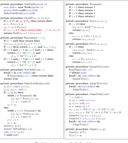
Firstly we must defineequivalence of 2chains. This definition relies on the functions Val+, Val−, which we invite the reader to consult at this point. (See Fig.4.) Briefly, a 2chain (1, x1, x2) is

equiv-alent to a 2chain (5, x5, x6) if and only if Val−(1, x1, x2, j) =xj forj = 5,6 or, equivalently, if and

only if Val+(5, x5, x6, j) =xj forj= 1,2. A 2chain (5, x5, x6) isequivalent to a 2chain (9, x9, x10) if and only if Val+₍₉_{, x}

9, x10, j) =xj forj= 5,6 or, equivalently, if and only if Val−(5, x5, x6, j) =xj

for j = 9,10. Moreover any 2chain is equivalent to itself. (Equivalence is defined in these specific cases only, and, in particular, we do not bother to extend the notion transitively, but which in any case would make no difference.) It can be noted that equivalence is time-dependent (like most of our definitions), in the sense that entries keep being added to the tablesFi.

Let (i, x) be a pending query. We will consider four cases according to the value of i. Let nbe the node such that n.end = (i, x). (We remind that such a node n exists and is unique; existence follows by definition of pending, uniqueness is argued within the proof.)

If i = 2, let x2 := x. A value x1 ∈ {0,1}n is a trigger for (i, x) = (i, x2) if F1(x1) 6= ⊥, if F10(x10) 6= ⊥ where (x10, x11) := P(x0, x1) where x0 := F1(x1)⊕x2, if F9(x9) 6= ⊥ where

x9 :=F10(x10)⊕x11, and finally if the 2chain (1, x1, x2) is not equivalent ton.idand not equivalent to c.id for any existing childc of n.

If i = 9, let x9 := x. A value x10 ∈ {0,1}n is a trigger for (i, x) = (i, x9) if F10(x10) 6= ⊥, if F1(x1) 6= ⊥ where (x0, x1) := P−1(x10, x11) where x11 := F10(x10)⊕x9, if F2(x2) 6= ⊥ where

x2 :=x0⊕F1(x1), and finally if the 2chain (9, x9, x10) is not equivalent ton.id and not equivalent to c.id for any existing childc of n.

If i= 5, letx5:=x. A valuex6 is atrigger for the pending query (i, x) = (i, x6) ifF6(x6)6=⊥ and if (5, x5, x6) is not equivalent to n.id and not equivalent to c.id for any existing child c ofn.

If i= 6, letx6:=x. A valuex5 is atrigger for the pending query (i, x) = (i, x6) ifF5(x5)6=⊥ and if (5, x5, x6) is not equivalent to n.id and not equivalent to c.id for any existing child c ofn.

The procedure that checks for triggers is FindNewChildren. Specifically, FindNewChildren takes as argument a node n, and checks if there exist triggers for the pending query7 n.end. For each

7_Let_n._end_{= (}_{i, x}_{). By definition, then, (}_{i, x}_{) is “pending” only if}_F

(17)

trigger y that FindNewChildren identifies, it creates a new child c for n; the id of c is set to (i−1, y, x) if i ∈ {2,6} and to (i, x, y) if i ∈ {5,9}. After creating c, FindNewChildren calls MakeNodeReady(c).

As a subtlety, one should observe that certain values y that are not triggers before a call to MakeNodeReady might be triggersafter the call. However one can also observe that FindNewChil-dren will in any case be called again on node n by virtue of having returned child added =true. (Indeed, GrowTree(root) only returns after doing a complete traversal of the tree such that no calls to FindNewChildren(·) during the traversal result in a new child.)

Partial Paths and Completed Paths. We define an (i, j)-partial path8 _{to be a sequence of} values xi, xi+1, . . . , xj if i < j, or a sequence xi, xi+1, . . . , x11, x0, x1, . . . , xj if i > j satisfying the

following properties:xh ∈Fh and xh−1⊕Fh(xh) =xh+1 for subscriptsh such thath /∈ {i, j,0,11}; if i > j, theni≤10,j≥1, andT(x0, x1) = (x10, x11); ifi < j, then 0≤i < j ≤11.

We notate the partial path as {xh}j_h₌_i regardless of whether i < j or i > j, with the

under-standing that x11 is followed by x0 ifi > j.

The values i and j are called the endpoints of the path. One can observe that two adjacent values xh, xh+1 on a partial path (h 6= 11) along with two endpoints (i, j) uniquely determine the partial path, if it exists.

An (i, j)-partial path{xh}jh=icontains a 2chain (ℓ, yℓ, yℓ+1) ifxℓ=yℓandxℓ+1 =yℓ+1; moreover if i=j+ 1, the caseℓ=j is excluded.

We say an (i, j)-partial path {xh}_hj₌_i is proper if i, j ∈[10], if xi ∈/ Fi,xj ∈/ Fj, and if (i, j) ∈

{(2,6),(5,9),(5,2),(6,2),(9,5),(9,6)}(the latter technical requirement is clarified in the proof, and needn’t be scrutinized now).

A completed path is a (0,11)-partial path{xh}11_h₌₀ such thatT(x0, x1) = (x10, x11).

The MakeNodeReady Procedure.Next we discuss the procedure MakeNodeReady. One can firstly observe that MakeNodeReady(node) is not called ifnodeis the root of its tree, as clear from the pseudocode. In particularnode.beginning6=null when MakeNodeReady(node) is called.

MakeNodeReady(node) behaves differently depending on whether the origin ofnode isi= 2,5,6 or 9. If i = 2 then node.id = (1, u1, u2) for some values u1, u2, where (i, u2) = node.beginning. Starting with j= 1, MakeNodeReady executes the instructions

(u1, u2)←Prev(j, u1, u2)

j←j−1 mod 11

untilj= 5. One can note (from the pseudocode of Prev) that after each call of the form Prev(j, u1, u2) with j 6= 0, Fj(u1) 6= ⊥. (When j = 0 the call Prev(j, u1, u2) entails a call to P−1 instead of to F.) Thus, after this sequence of calls, there exists a partial path x5, x6, . . . , x1, x2 with endpoints (i, j) = (2,5) and with (1, x1, x2) =node.id.

We also haveF2(x2) =⊥by item 4 above and, if MakeNodeReady doesn’t abort,F5(x5) =⊥as well when MakeNodeReady returns. In particular, x5, x6, . . . , x1, x2 is a proper (5,2)-partial path when MakeNodeReady returns, containing node.id.

For i = 5, MakeNodeReady similarly creates a (5,2)-partial path x5, x6, . . . , x1, x2 such that (5, x5, x6) = node.beginning, by repeated calls to Next. Here the partial path is also proper when MakeNodeReady returns, and likewise contains node.id.

(18)

The cases i= 6 and i= 9 are symmetric, respectively, to the cases i= 5 and i= 2.

In summary, when MakeNodeReady(node) returns one has node.beginning6=null, node.end6= null, and there exists a proper (i, j)-partial pathxi, xi+1, . . . , x11, x0, . . . , xj containingnode.idsuch

that (i, j)∈ {(5,2),(9,6)} and such that

{(i, xi),(j, xj)}={node.beginning,node.end}.

Path Completion Process.We say that nodenisstableif no triggers exist for the queryn.end. When GrowTree(root) returns in NewTree, each node in the tree rooted at root is both ready and stable. (This is rather easy to see syntactically from the pseudocode.) Moreover each non-root node of the tree is associated to a partial path, which is the unique partial path containing that node’s id and whose endpoints are the node’s origin and terminal.

After GrowTree(root) returns, SampleTree(root) is called, which calls ReadTape(i, x) for each (i, x) such that (i, x) =n.end for some node nin the tree rooted at root. This effectively assigns a uniform independent random value toFi(x) for each such pair (i, x).

One can observe that the only nodes whose stability is potentially affected by a change to the table F5 (resp. F6) are nodes with terminal 6 (resp.5). Likewise, the only nodes whose stability is potentially affected by a change to the table F2 (resp. F9) are nodes with terminal 9 (resp. 2). Given that all the nodes in the tree either have terminalsi∈ {2,5}or terminalsi∈ {6,9}, the calls to ReadTape that occur in SampleTree(root) do not affect the stability of the nodes the current tree, i.e., the tree rooted atroot. (On the other hand the stability of nodes of trees higher up in the stack is potentially affected.)

After SampleTree(root) returns, AdaptTree(root) is called, which “adapts” the partial path associated9 _{to each non-root node of the tree into a completed path. In more detail, if the endpoints} of the partial paths are 2 and 5 then F3 and F4 are adapted (by a call to the procedure ‘Adapt’) as in equations (1) and (2); if the endpoints of the partial paths are 6 and 9 then F7 and F8 are adapted, via similar assignments.

Further Pseudocode Details: The TablesTsim/Tsim−1.In order to reduce its query complexity, and following an idea of [11], our simulator keeps track of which queries it has already made to P or P−1 via a pair of tables Tsim and Tsim−1. These tables are maintained by the procedures SimP and SimP−1 _(Fig_._{3), which are “wrapper functions” that the simulator uses to access P and P}−1_. If the simulator did not use the tables Tsim and T_sim−1 to remember its queries to P/P−1, the query complexity would be quadratically higher:O(q8) instead ofO(q4). (This is the route taken by [17], and their query complexity could be indeed be lowered from O(q8_{) to} _O₍_q4_{) by using the trick of} remembering past queries to P/P−1.)

We also note that the tables Tsim,Tsim−1 are accessed by the procedures Val+ and Val− of game G1 (see Fig. 5), while in games G2–G4 Val+ and Val− access the tables T and T−1 directly, which are not accessible to the simulator in game G1. As it turns out, games G1–G4 would be unaffected if the procedures Val+, Val− called SimP/SimP−1 (or even P/P−1) instead of doing table look-ups “by hand”, because it turns out that Val+_{, Val}−_{never return}_⊥_{in any of games G}

1–G4(see Lemma 21); but we choose the latter presentation (i.e., accessing the tablesTsim/T_sim−1 orT/T−1, depending) in order to emphasize—and to more easily argue within the proof—that calls to Val+, Val− do not cause “new” queries to P/P−1_.

(19)

5 Proof of Indifferentiability

In this section we give a proof for Theorem 1, using the simulator described in Section 4 as the indifferentiability simulator.

In order to prove that our simulator successfully achieves indifferentiability as defined by Def-inition 1, we need to upper bound the time and query complexity of the simulator, as well as the advantage of any distinguisher. These three bounds are the objects of Theorems 34, 31 and 84 respectively.

Game Sequence.Our proof uses a sequence of five games, G1, . . . , G5, with G1being the simulated world and G5 being the real world. Games G1–G4 are described by the pseudocode of Figs. 3–6 while game G5 is given by the pseudocode of Fig. 7. Every game offers the same interface to the distinguisher, consisting of functions F, P and P−1.

A brief synopsis of the changes that occur in the games is as follows:

In G2: The simulator’s procedure CheckP (Fig.4) used by the simulator in FindNewChildren (Fig.3) “peeks” at the tableT and returns⊥if (x0, x1)∈/ T; this modification ensures that a call to CheckP does not result in a “fresh” call to P. Also, the procedures Val+_{, Val}− _{use the tables} _T_,

T−1 instead ofTsim,Tsim−1. (As mentioned at the end of the last section, the second change does not actually alter the behavior of Val+, Val−, despite the fact that the tablesTsim,Tsim−1 may be proper subsets of the tablesT,T−1_{(see Lemma 21). On the other hand, the change to CheckP may result} in “false negatives” being returned by CheckP.)

In G3: The simulator adds a number of checks that may cause it to abort in places when it did not abort in G2. Some of these involve peeking at the random permutation table T, which means they cannot be included in G1. Otherwise, G3 is identical to G2, so the only difference between G2 and G3 is that G3 may abort when G2 does not. The pseudocode for the new checking procedures called by G3 are in Fig. 8.

In G4: The only difference occurs in the implementation of the oracles P, P−1(see Fig.6). In G4, these oracles no longer rely on the random permutation table p :{0,1}2n _{→ {0}_,_1}2n_{, but instead}

evaluate a 10-round Feistel network using the random tapes f1, . . . , f10 as round functions.

In G5: This is the real world, meaning that F(i, x) directly returns the value fi(x). As will be

shown in the proof, the only “visible” difference between G4 and G5 is that G4 may abort, while G5 does not.

The advantage of a distinguisher D at distinguishing games Gi and Gj is defined as ∆D(Gi,Gj) = Pr

Gi

[DF,P,P−1 = 1]−Pr Gj

[DF,P,P−1 = 1] (3)

where the probabilities are taken over the coins of the relevant game as well as over D’s coins, if any. Most of the proof is concerned with upper bounding∆D(G1,G5) for a distinguisher Dthat is limited to q queries (in a nonstandard sense defined below); the simulator’s efficiency, as well its query complexity (Theorems 34 and 31 respectively) will be established as byproducts along the way.

(20)

acknowledging the extra power of the distinguisher actually helps to improve the final bound, as we shortly explain.

SinceDis information-theoretic, we can assume without loss of generality thatDis deterministic by fixing the best possible sequence of coin tosses forD. (See, e.g., the appendix in the proceedings version of [6].)

We can also assume without loss of generality thatDoutputs 1 if an oracle abort. Indeed, since the real world G5 does not abort, this can only increase the distinguishing advantage∆D(G1,G5). Some of our lemmas, moreover, only hold ifDis a distinguisher thatcompletes all paths, as per the following definition:

Definition 1. A distinguisherDcompletes all pathsif at the end of every non-aborted execution,D

has made the queries F(i, xi) fori= 1,2, . . . ,10 wherexi = F(i−1, xi−1)⊕xi−2 fori= 2,3, . . . ,10, for every pair (x0, x1) such thatDhas either queried P at (x0, x1) at some point during the execution or such that P−1 returned (x0, x1) to Dat some point during the execution.

Lemmas that only hold if D completes all paths (and which are confined to sections 5.5, 5.7) are marked with a (*).

It is not difficult to see that for every distinguisherDthat makes at mostq queries to each of its oracles, there is a distinguisherD∗ _{that completes all paths, that achieves the same distinguishing} advantage as D, and that makes at most 2q queries to each of its oracles. Hence, the cost of assuming a distinguisher that completes all paths is a factor of two in the number of queries. (Previous papers [1, 17, 19] pay for the same assumption by giving r times as many queries to the distinguisher, where r is the number of rounds. Our trick of explicitly giving the distinguisher the power to query each of its oraclesq times reduces this factor to 2 without harming the final bound; indeed, current proof techniques effectively give the distinguisher q queries to each of its oracles anyway. Our trick also partially answers a question posed in [1].)

Miscellaneous.Unless otherwise specified, anexecution refers to a run of one of the games G1, G2, G3, G4 (excluding, thus, G5) with the fixed distinguisherD mentioned above.

5.1 Efficiency of the Simulator

We start the proof by proving that the simulator is efficient in games G1 through G4. This part is similar to previous efficiency proofs such as [11, 17], and ultimately relies on Seurin’s termination argument, outlined at the end of Section 3.

Unless otherwise specified, lemmas in this section apply to games G1 through G4. As the proof proceeds, and for ease of reference, we will restate some (but not all) of the definitions made in Section 4.

Definition 2. A query (i, xi) is defined if Fi(xi) 6=⊥. It is pending if it is not defined and there

exists a noden such thatn.end= (i, xi).

Definition 3. A completed path is a sequence x0, . . . , x11 such that xi+1 = xi−1 ⊕Fi(xi) for

1≤i≤10 and such that T(x0, x1) = (x10, x11).

Definition 4. A node n is created if its constructor has returned. It is ready if n.end = (i, xi)6=

(21)

We emphasize that a completed node is also a sampled node, that a sampled node is also a ready node, etc. We thus have the following chain of containments:

created nodes⊇ready nodes⊇sampled nodes⊇completed nodes

We also note that a root noder cannot become completed becauser.id=null(and remainsnull) for root nodes. Moreover, we remind that nodes are never deleted (even after the last reference to a node is lost).

Lemma 1. The parent, id, beginning, and end fields of a node are never overwritten after they are assigned a non-null _value.

Proof. This is easy to see from the pseudocode. The parent, id and beginning of a node are only assigned in the constructor. The only two functions to edit theendfield of a node are NewTree and MakeNodeReady. NewTree creates a root with a null end field and immediately assigns the end

field to a non-nullvalue, while MakeNodeReady(n) is only called for nodes n that are not roots, and is called at most once for each node.

Lemma 2. A node is a root node if and only if it is a root node after its constructor returns, and if and only if it is created in the procedure NewTree.

Proof. Recall that by definition a nodenis a root node if and only ifn.beginning=null. The first “if and only if” therefore follows from the fact that the beginning field of a node is not modified outside the node’s constructor.

The second “if and only if” follows by inspection of the procedures NewTree (Fig. 3) and AddChild (Fig.4), which are the only two procedures to create nodes.

The above lemmas show that all fields of a node are invariant after the node’s definition, except for the set of children, which grows as new paths are discovered. Therefore when we refer to these variables in the following discussions, we don’t need to specify exactly what time we are talking about (as long as they are defined).

Lemma 3. The entries of the tablesFi are not overwritten after they are defined.

Proof. The only two procedures that modify tablesFiare ReadTape and Adapt. In both procedures

the simulator checks that xi ∈/ Fi (and aborts if otherwise) before assigning a value toFi(xi).

Lemma 4. Entries in tables T and T−1 _{are never overwritten and} _T

sim (T_sim−1) is a subset of T (T−1). Moreover, in games G1,G2and G3,T andT−1 are compatible with the permutation encoded

by tape p and its inverse.

Proof. The tables T and T−1 are only modified in P or P−1. Entries are added according to a permutation, which is the permutation encoded by the random tape p in G1, G2 and G3, and is the 10-round Feistel network built from the round functions (random tapes) f1, . . . , f10 in G4. By inspection of the pseudocode, the entries are never overwritten.

The table Tsim is only modified in SimP and SimP−1. The entry added toTsim is obtained via a call to P or P−1_{, where the corresponding entry in} _T _{is returned, and hence the same entry also} exists inT.

(22)

Proof. A node becomes ready when its end is assigned a query. This only occurs in NewTree and MakeNodeReady, and in both cases the node is added intoN immediately after the assignment. Lemma 6. Let n be a ready node with n.end = (i, xi). Then IsPending(i, xi) = true or xi ∈Fi from the moment when nis added to N until the end of the execution.

Proof. The procedure IsPending(i, xi) returnstrue while n is inN. Note that n is removed from N only in SampleTree, right after ReadTape(n.end). Therefore, at the moment whennis removed from N we already have xi ∈Fi. Since entries in Fi are not overwritten, this remains true for the

rest of the execution.

Lemma 7. We have n1.end6=n2.end for distinct nodes n1 andn2 with n1.end6=null.

Proof. Assume by contradiction that there exist two nodes n1, n2 such that n1.end = n2.end = (i, xi). Without loss of generality, supposen1 becomes ready before n2.

If n2 is the root of a tree, it becomes ready after it is created in NewTree, called by F(i, xi).

Between the time when F(i, xi) is called and the time NewTree executes its second line, no

modifi-cation is made to the other nodes, son1is already ready when the call F(i, xi) occurs. By Lemmas 5

and 6, when F(i, xi) is called, we have IsPending(i, xi) = true or xi ∈ Fi. But F(i, xi) aborts if

IsPending(i, xi) = true, and it returns Fi(xi) directly if xi ∈ Fi. NewTree is not called in either

case, leading to a contradiction.

If n2 is not a root node, itsend is assigned in MakeNodeReady. Before n2.end is assigned, two assertions are checked. Since no modification is made to the other nodes during the assertions,n1 is ready before the assertions. By Lemmas 5 and 6, we must have IsPending(i, xi) =true(violating

the second assertion) or xi ∈Fi (violating the first assertion). In both cases the simulator aborts

before the assignment, which is also a contradiction.

Lemma 8. FindNewChildren(n) is only called if n is a ready node.

Proof. Recall that ready nodes never revert to being non-ready (cf.Lemma 1).

If nis created by NewTree thenn.endis assigned by NewTree immediately after creation, and hence nis ready.

Ifnis created by AddChild, on the other hand, then AddChild calls MakeNodeReady(n) imme-diately, which does not return until n is ready. Moreover, while MakeNodeReady(n) calls further procedures, it does not pass on a reference tonto any of the procedures that it calls, so it is impos-sible for a call FindNewChildren(n) to occur while MakeNodeReady(n) has not yet returned. Lemma 9. A node n is a child of n′ if and only if n.beginning=n′.end6=null.

Proof. If n′ ₌ _n._parent_{, then in the constructor of} _n_{, its} _beginning _{is assigned the same value as}

n′.end. Since FindNewChildren is only called on ready nodes, n′.end 6= null. By Lemma 1, both

n.beginning and n′.end are not overwritten, thus n.beginning =n′.end6=null until the end of the execution.

On the other hand, if n.beginning=n′.end6=null, thennis a non-root node. As proved in the “if” direction, we must have n.parent.end =n.beginning =n′.end. By Lemma 7, the end of ready nodes are distinct, thusn.parent=n′_.

(23)

Proof. The end of a node is only assigned in NewTree and MakeNodeReady. NewTree(i, xi) is

only called by F(i, xi) for i ∈ {2,5,6,9}. When the end of a node is assigned a query (j, xj) in

MakeNodeReady, we havej= Terminal(i), while the output of Terminal is 2, 5, 6 or 9.

A query can be defined a call to procedures F, Adapt, and SampleTree. F calls ReadTape only if i /∈ {2,5,6,9}, and Adapt is only called on queries in positions 3, 4, 7 and 8. Therefore, queries in positions 2, 5, 6 and 9 must be defined (if at all) in SampleTree.

Lemma 11. For every node n, the query n.end is not defined until SampleTree(n) is called. Proof. By Lemma 10, n.end is in position 2, 5, 6 or 9, and must be sampled in a call to Sample-Tree(n′) for some noden′. The query defined in SampleTree(n′) isn′.end. By Lemma 7, if n′ 6=n,

n′_._end₆₌_n._end_{. Therefore, the query}_n._end_{must be defined inside of SampleTree(}_n_).

Lemma 12. The setN consists of all nodes that are ready but not sampled, except for the moments right before a node is added to N or right before a node is deleted from N.

Proof. By Lemma 5, a node is added toN right after it becomes ready. On the other hand, a node is added to N only in procedures NewTree and MakeNodeReady, and in both procedures the end

of the node is assigned a non-nullvalue before it is added.

Then we only need to prove that a node is removed from N if and only if it becomes sampled. A nodenis deleted from N only in the procedure SampleTree. ReadTape is called onn.endbefore the deletion, so the node is sampled when the deletion occurs. Moreover, by Lemma 11, the query

n.end can only be defined in SampleTree(n), following which the deletion occurs immediately. Therefore, the setN always equals the set of nodes that are ready but not sampled, except for the gaps between the two lines when the sets are changed.

Lemma 13. At all points when calls to IsPending occur in the pseudocode, the call IsPending(i, xi) returns true if and only if the query (i, xi) is pending.

Proof. IsPending(i, xi) returns true if and only if there exists a node n in N such that n.end =

(i, xi). Since IsPending is not called immediately before a modification toN, Lemma 12 implies that

this occurs if and only if there exists a nodensuch thatn.end= (i, xi) and such thatFi(xi) =⊥.

Definition 5. Let ˜Fidenote the set of queries in positionithat are pending or defined, fori∈[10].

For any i∈[10], since Fi is the set of defined queries in positioni, we have Fi ⊆F˜i. The sets ˜Fi

are time-dependent, like the setsFi.

Lemma 14. The sets F˜i are monotone increasing, i.e., once a query becomes pending or defined, it remains pending or defined for the rest of the execution.

Proof. By Lemma 3, we know that after an entry is added to a table, it will not be overwritten. Therefore any defined query will remain defined through the rest of the execution.

For each pending query (i, xi), there exists a node n such that (i, xi) = n.end. By Lemma 1, n.end will not change and thus (i, xi) must be pending if it is not defined.

(24)

Proof. Observe that in each call to NewTree, SampleTree is called on every node in the tree before NewTree returns, unless the simulator aborts. Therefore, all pending queries in the tree become defined before NewTree successfully returns. A non-aborted query cycle ends only after all calls to NewTree have returned, so all pending queries are defined by then.

Next we upper bound the number of nodes created by the simulator and the sizes of the tables. We will separate the nodes into two types as in the following definition, and upper bound the number of each type. Recall that in the simulator overview we defined theorigin andterminal of a non-root node nto be the positions of n.beginning andn.endrespectively.

Definition 6. A non-root node is an outer nodeif its origin is 2 or 9, and is an inner nodeif its origin is 5 or 6.

The names imply by which detect zone a path is triggered: an inner node is associated with a path triggered by the middle detect zone; an outer node is associated with a path triggered by the outer detect zone.

Lemma 16. The number of outer nodes created in an execution is at most q.

Proof. It is easy to see from the pseudocode that before an outer node is added in FindNewChildren, the counter NumOuteris incremented by 1. The simulator aborts when the counter exceeds q, so the number of outer nodes is at most q.

Now we give a formal definition of partial path, superseding (or rather augmenting) the definition given in Section 4.

Definition 7. An (i, j)-partial path is a sequence of values xi, xi+1, . . . , xj if i < j, or a sequence xi,xi+1,. . . , x11, x0, x1, . . . , xj if i > j, satisfying the following properties:i6=j and 0≤i, j ≤11; xh ∈ Fh and xh−1⊕Fh(xh) = xh+1 for subscripts h such that h /∈ {i, j,0,11}; if i > j, we also require (i, j) 6= (11,0), T(x0, x1) = (x10, x11) if 1≤j < i ≤10, T(x0, x1) = (∗, x11) if i= 11, and

T−1₍_x

10, x11) = (x0,∗) ifj= 0.

As can be noted, the only difference with the definition given in Section 4 is that the cases i= 11 and j= 0 (though not both simultaneously) are now allowed.

Let {xh}j_h₌_i be an (i, j)-partial path. Each pair (h, xh) with h∈ {i, i+ 1, . . . , j} if i < j, or with

h∈ {i, i+ 1, . . . ,11} ∪ {0,1, . . . , j}

if i > j is said to be in the partial path. We also say the partial path contains (h, xh). We may

also say that xh is in the partial path (or that the partial path contains xh) without mentioning

the indexh, if his clear from the context.

Note that a partial path may contain pairs of the form (11, x11) and (0, x0) even though such pairs aren’t queries, technically speaking.

As previously, a partial path {xh}jh=i contains a 2chain (ℓ, xℓ, xℓ+1) (with 0≤ℓ≤10) if (ℓ, xℓ)

and (ℓ+ 1, xℓ+1) are both in {xh}j_h₌_i and if ℓ6=j.