Pushover Analysis Of Building With Or With Out Shear Walls

(1)

Available online: https://edupediapublications.org/journals/index.php/IJR/ P a g e | 2755

Pushover Analysis Of Building With Or With Out Shear Walls

N.Murali Krishna1_{, G.Narender2, J.Mounika}3

1

(Assistant Professor, Civil Engineering, Anurag Engineering College) 2

(Assistant Professor, Civil Engineering, Anurag Engineering College) 3

(Assistant Professor, Civil Engineering, Anurag Engineering College)

INTRODUCTION Abstract

A performance - based design is at controlling the structural damage based on precise estimation of proper response parameter. In performance based seismic analysis evaluates how building is likely to perform. It is an iterative process with selection of performance objective followed by development of preliminary design, an assessment whether or not the design meets the performance objective; In the present study pushover analysis has been done an two multistoried R.C. frame building; In which plan of one building was taken symmetrical and it consist of 2 bay of 5m in x direction & 2 bay of 4m in y direction and second building having L shaped unsymmetrical plan. The shear wall is providing for studying their resisting lateral forces. In this paper highlight the effect of shear wall on R.C frame building when shear wall providing along the longer and shorter side of the building. The base shear and displacement will decreases of building. The comparative study has been done for base shear, story drift, spectral acceleration, spectral displacement, story displacement. The Concept of seismic design is to provide building structure with sufficient strength and deformation capacity to sustain seismic demands imposed by ground motion with adequate margin of safety. Even if the probability of occurrence of earthquake within the life span of structures is very less, strong ground motion would generally cause greater damage to the structure. For designing the structures for this combination having less probability and extreme loading, a criterion is adopted in such a way that a major earthquake, with a relatively low probability of occurrence is expected to cause significant damage which may not be repairable but not associated with loss of life Performance based seismic design is gaining popularity from last decades. Many countries are separate document over this method such as

FEMA, ATC etc. Recently formulated Euro codes EC2 and EC8 [Euro code 2, Euro code 8] are also based on performance based design philosophy. But Indian codes are still silent over this method.

GENERAL

Seismic analysis is a subset of structural analysis and is the calculation of the response of

a building (or non-building) structure

to earthquakes. It is part of the process of structural design, earthquake engineering or structural assessment and retrofit in regions where earthquakes are prevalent.

As seen in the figure, a building has the potential to ‘wave’ back and forth during an earthquake (or even a severe wind storm). This is called the ‘fundamental mode’ and is the

lowest frequency of building response.

However, most buildings have higher modes of response, which are uniquely activated during earthquakes. The figure just shows the first and second mode, but there are higher ‘shimmy’ (abnormal vibration) modes. Nevertheless, the first and second modes tend to cause the most damage in most cases.

Figure 1.1 First and second modes of building seismic response

Structural analysis methods can be divided into the following five categories.

a) Linear static analysis b) Linear dynamic analysis c) Non linear static analysis d) Non linear dynamic analysis Linear static analysis

(2)

Available online: https://edupediapublications.org/journals/index.php/IJR/ P a g e | 2756 stiffness and an equivalent viscous damping.

The seismic input is modeled by an equivalent lateral force with the objective to produce the same stresses and strains as the earthquake it represents. Based on an estimation of the first fundamental frequency of the building using empirical relationships or Rayleigh’s method, the spectral acceleration is determined from the appropriate response spectrum which, multiplied by the mass of the building, results in the equivalent lateral force. The coefficients take into account issues like second order effects, stiffness degradation, but also force reduction due to anticipated inelastic behavior. The lateral force is then distributed over the height of the building and the corresponding internal forces and displacements are determined using linear elastic analysis.

Linear dynamic analysis

Static procedures are appropriate when higher mode effects are not significant. This is generally true for short, regular buildings. Therefore, for tall buildings, buildings with torsion irregularities, or non-orthogonal systems, a dynamic procedure is required. In the linear dynamic procedure, the building is modeled as a multi-degree-of-freedom (MDOF) system with a linear elastic stiffness matrix and an equivalent viscous damping matrix.

Non-linear static analysis

In general, linear procedures are applicable when the structure is expected to remain nearly elastic for the level of ground motion or when the design results in nearly uniform distribution of nonlinear response throughout the structure. As the performance objective of the structure implies greater inelastic demands, the uncertainty with linear procedures increases to a point that requires a high level of conservatism in demand assumptions and acceptability criteria to avoid unintended performance. Therefore, procedures incorporating inelastic analysis can reduce the uncertainty and conservatism.

Figure 1.2 Hinge performance levels

Force-displacement or moment-rotation curve for a hinge definition used in ETABS (plastic-deformation curve). The plastic (plastic-deformation curve is characterized by the following points:

 Point A represents the origin.

 Point B represents the yielding state. No deformation occurs in the hinge up to point B, regardless of the deformation value specified for point B. The displacement (rotation) at point B will be subtracted from the deformations at points C, D, and E. Only the plastic deformation beyond point B will be exhibited by the hinge.

 Point C represents the ultimate capacity for pushover analysis.

 Point D represents the residual strength for pushover analysis.

 Point E represents total failure. Beyond point E the hinge will drop load down to point F (not shown) directly below point E on the horizontal axis. If the users do not want the hinge to fail this way, a large value for the deformation at point E can be specified.

SHEAR WALLS INTRODUCTION

Shear walls are vertical elements of the horizontal force resisting system. The reinforced concrete shear wall is important structural elements placed in multi-storey buildings which are situated in seismic zones because they have a high resistance to lateral earthquake loads. RC shear walls must have sufficient ductility to avoid brittle failure under the action of strong lateral seismic loads. In residential construction, shear walls are straight external walls that typically form a box which provides all of the lateral support for the building. When shear walls are designed and constructed properly, and they will have the strength and stiffness to resist the horizontal forces.

(3)

Available online: https://edupediapublications.org/journals/index.php/IJR/ P a g e | 2757 Figure 3.1 Reinforced concrete shear walls in

buildings

PURPOSE OF CONSTRUCTING SHEAR WALLS

Shear walls are not only designed to resist gravity / vertical loads (due to its self-weight and other living / moving loads), but they are also designed for lateral loads of earthquakes / wind. The walls are structurally integrated with roofs / floors (diaphragms) and other lateral walls running across at right angles, thereby giving the three dimensional stability for the building structures. Shear wall structural systems are more stable. Because, their supporting area (total cross-sectional area of all shear walls) with reference to total plans area of building, is comparatively more, unlike in the case of RCC framed structures. Shear walls have to resist the uplift forces caused by the pull of the wind. Shear walls have to resist the shear forces that try to push the walls over. Walls have to resist the lateral force of the wind that tries to push the walls in and pull them away from the building. Shear walls are quick in construction, as the method adopted to construct is concreting the members using formwork. Shear walls doesn’t need any extra plastering or finishing as the wall itself gives such a high level of precision, that it doesn’t require plastering. CLASSIFICATION OF SHEAR WALLS

 Simple rectangular types and flanged walls

 Coupled shear walls

 Framed walls with in filled frames  Core type shear walls

Simple rectangular types and flanged walls These simple types were the first be used in construction. Such shear walls, under the action of in plane vertical loads and horizontal shear along its length, are subjected to bending and shear. Uniform distribution of steel over as is used in the simple shear walls is not as efficient as putting the minimum steel over the inner 0.7 to 0.8 length L of the wall and placing the remaining steel at the ends for a length 0.15 0.12 L on either side.

Figure 3.2 Different types of flanged type shear walls

Coupled shear walls

Coupled shear walls consist of two shear walls connected intermittently by beams along the height. The behavior of coupled shear walls is mainly governed by the coupling beams. The coupling beams are designed for ductile inelastic behavior in order to dissipate energy. The base of the shear walls may be designed for elastic or ductile inelastic behaviors. The amount of energy dissipation depends on the yield moment capacity and plastic rotation capacity of the coupling beams.

Figure 3.3 Typical coupled shear wall METHODOLOGY

PUSHOVER ANALYSIS – AN OVERVIEW The use of the nonlinear static analysis (pushover analysis) came in to practice in 1970‟s but the potential of the pushover analysis has been recognized for last two decades years. This procedure is mainly used to estimate the strength and drift capacity of existing structure and the seismic demand for this structure subjected to selected earthquake. This procedure can be used for checking the adequacy of new structural design as well. The effectiveness of pushover analysis and its computational simplicity brought this procedure in to several seismic guidelines (ATC 40 and FEMA 356) and design codes (Euro code 8 and PCM 3274) in last few years.

 Estimates of force and displacement capacities of the structure. Sequence of the member yielding and the progress of the overall capacity curve.

 Estimates of force (axial, shear and moment) demands on potentially brittle elements and deformation demands on ductile elements.

 Estimates of global displacement demand, corresponding inter-storey drifts and damages on structural and non-structural

elements expected under the 20

earthquake ground motion considered.  Sequences of the failure of elements and

(4)

Available online: https://edupediapublications.org/journals/index.php/IJR/ P a g e | 2758  Identification of the critical regions, when

the inelastic deformations are expected to be high and identification of strength irregularities (in plan or in elevation) of the building.

Pushover analysis delivers all these benefits for an additional computational effort (modeling nonlinearity and change in analysis algorithm) over the linear static analysis. Step by step procedure of pushover analysis is discussed next.

PURPOSE OF PUSHOVER ANALYSIS The purpose of pushover analysis is to evaluate the expected performance of structural systems by estimating performance of a structural system by estimating its strength and deformation demands in design earthquakes by means of static inelastic analysis, and comparing these demands to available capacities at the performance levels of interest. The evaluation is

based on an assessment of important

performance parameters, including global drift, inter story drift, inelastic element deformations (either absolute or normalized with respect to a yield value), deformations between elements, and element connection forces (for elements and connections that cannot sustain inelastic deformations). The following are the examples of such response characteristics:

 The realistic force demands on potentially brittle elements, such as axial force demands on columns, force demands on brace connections, moment demands on beam to column connections, shear force demands in deep reinforced concrete spandrel beams, shear force demands in unreinforced masonry wall piers, etc.  Estimates of the deformations demands

for elements that have to form in-elastically in order to dissipate the energy imparted to the structure.

 Consequences of the strength deterioration of individual elements on behavior of structural system.

INTRODUCTION TO LOAD PATTERN Nonlinear static analysis or pushover analysis could be performed directly by a computer program which can model nonlinear behavior of lateral load resisting members of a structure. However, the computational scheme and the assumptions involved in modeling nonlinear member behavior could be different that there

may be variation in the pushover results obtained from different software. Therefore, the underlying principles of any software utilized for pushover analysis should be well understood to interpret the results of pushover analysis.

Description of the terms used in pushover analysis window

A pushover case may start from zero initial condition, or it may start from the end of a previous pushover case. However, ETABS v9.7.3 allows plastic hinge formation during ‘gravity’ pushover analysis. ETABS v9.7.3 can also perform pushover analysis as either force-controlled or displacement-force-controlled. The “Push to Load Level Defined by Pattern” option button is used to perform a force-controlled analysis. The pushover typically proceeds to the full load value defined by the sum of all loads included in the “Load Pattern” box (unless it fails to converge at a lower force value). “The Push to Displacement Magnitude” option button is used to perform a displacement-controlled analysis. The pushover typically proceeds to the specified displacement in the specified control direction at the specified control joint (unless it fails to converge at a lower displacement value).

Element description of ETABS v9.7.3

In ETABS V9.7.3, a frame element is modeled as a line element having linearly elastic properties and nonlinear force-displacement characteristics of individual frame elements are modeled as hinges represented by series of straight line segments a generalized force displacement characteristic of a non-degrading frame element (or hinge properties) in ETABS V 9.7.3 is shown figure 5.3 a point corresponds 6to unloaded condition and point B represents yielding of the element.

STRUCTURAL PERFORMANCE LEVELS AS PER FEMA 273

According to FEMA-273, the structural

performance levels and damage states are detailed in the Table below. The drift values given in table are typical values provided to illustrate the overall structural response associated with various performance levels.

Table 4.1 Structural Performance Levels

Type Immediate

Occupanc y

Life Safety

(5)

Available online: https://edupediapublications.org/journals/index.php/IJR/ P a g e | 2759 Primar

y damage

Minor hair line cracking. No Crushing.

Extensiv e damage to beams. Sapling of cover and shear cracking.

Extensive cracking and hinge formation in ductile elements. Severe damage in short columns.

Drift 1%

transient.

2% transient.

4% transient.

RESULTS AND DISCUSSIONS GENERAL

In this chapter, the structure is modeled for 10 and 15 storied building considered in zone V which is symmetrical in plan. A non-linear static analysis is performed in ETABS v9.7.3 and the results are generated in the form of pushover curves which are presented here. The same building is analyzed by taking symmetric

condition and analyzed after applying

retrofitting.

RESULTS OBTAINED FOR A 10-STORIED BUILDING

Observations under pushover curve

The structure was given initial drift about 1%

which was calculated to be equal to

[{32x(1/100)}=0.32] 320mm and the pushover curve for the structure was graphically generated as shown in figure and for the 1% drift with shear wall the maximum base shear was observed to be 27014.48kN as observed in table 6.1

Table 6.1 shows base shear, roof displacement and the number of elements falling in different performance zones like immediate occupancy, life safety collapse prevention. It was observed from the Table 6.1 that the hinges for the structure were in the elastic region (i.e. A to B) up to a displacement of 32mm and further increase in the displacement leads to formation of 2 hinges with this the structure enters in to the nonlinear stage (i.e. B to IO ). The number of hinge formation for the structure remains in this

“Immediate Occupancy” level till the

displacement reached 32mm with base shear of

3912.91kN. The structure enters the

performance level “life safety” with the formation of hinges of 2 hinges at the displacement of about 82mm the building remained in the life safety level. The structure enters in the collapse prevention level after further increases in displacement till 314mm it was with the help of 111 additional hinges. Table 6.1 Pushover curve for a 10-storied symmetrical building for drift 1%

Displacement Base

Force A-B B-IO

IO-LS

LS-CP CP-C C-D D-E >E TOTAL 0 0 1430 0 0 0 0 0 0 0 1430 0.032 3912.92 1428 2 0 0 0 0 0 0 1430 0.049 5996.76 1303 127 0 0 0 0 0 0 1430 0.082 9715.25 1112 316 2 0 0 0 0 0 1430 0.116 12678 1025 359 46 0 0 0 0 0 1430 0.1503 15329.3 984 361 85 0 0 0 0 0 1430 0.1835 17782.2 956 255 181 38 0 0 0 0 1430 0.2213 20519.7 914 244 212 60 0 0 0 0 1430 0.256 22988.8 892 231 235 72 0 0 0 0 1430 0.2898 25346.1 870 222 240 96 0 2 0 0 1430 0.3144 27061.7 870 220 241 97 0 0 2 0 1430 0.3144 27014.5 868 217 232 111 0 0 2 0 1430 0.32 27438.5 1430 0 0 0 0 0 0 0 1430 Observations under capacity spectrum curve

Table 6.2 shows the capacity spectrum curve for a drift of 0.32m, obtained from the intersection of pushover curve with response spectrum curve. Both these curves are converted in terms of spectral acceleration and spectral displacement

i.e. in the Acceleration-displacement response spectrum (ADRS) format, and then are superimposed to give the performance point of the structure. The effective period is at a performance point is 0.996 sec which can be seen in step 3 and 4.

Table 6.2 Capacity spectrum curve for a 10-storied symmetrical building for drift 1%

(6)

Available online: https://edupediapublications.org/journals/index.php/IJR/ P a g e | 2760 RESULTS OBTAINED FOR A 10-STORIED

BUILDING

[{64x(1/100)}=0.64] 640mm and the pushover

curve for the structure was graphically generated as shown in figure and for the 2% drift with shear wall the maximum base shear was observed to be 28189.72kN as observed in table 6.3.

Table 6.3 Pushover curve for a 10-storied symmetrical building for drift 2%

Observations under capacity spectrum curve Table 6.4 shows the capacity spectrum curve for a drift of 0.32m, obtained from the intersection of pushover curve with response spectrum curve. Both these curves are converted in terms of spectral acceleration and spectral displacement

i.e. in the Acceleration-displacement response spectrum (ADRS) format, and then are superimposed to give the performance point of the structure. The effective period is at a performance point is 0.997 sec which can be

seen in step 1 and 2

.

Step Teff ßeff Sd(C) Sa(C) Sd(D) Sa(D) ALPHA PF*Ø

0 0.932 0.05 0 0 0.093 0.429 1 1

1 0.932 0.05 0.033 0.152 0.093 0.429 0.699 1.496

2 0.98 0.07 0.076 0.318 0.089 0.375 0.697 1.499

3 1.037 0.091 0.119 0.444 0.088 0.328 0.694 1.502

4 1.074 0.096 0.163 0.568 0.089 0.312 0.692 1.504

5 1.099 0.096 0.206 0.686 0.091 0.305 0.691 1.505

0 0.932 0.05 0 0 0.093 0.429 1 1 1 0.932 0.05 0.021 0.099 0.093 0.429 0.699 1.496 2 0.932 0.05 0.033 0.152 0.093 0.429 0.699 1.496 3 0.947 0.058 0.055 0.246 0.091 0.407 0.699 1.496 4 0.983 0.078 0.077 0.322 0.087 0.362 0.697 1.5 5 1.016 0.09 0.1 0.391 0.086 0.336 0.695 1.501 6 1.04 0.096 0.122 0.454 0.087 0.323 0.694 1.503 7 1.063 0.098 0.147 0.525 0.088 0.314 0.693 1.504 8 1.079 0.098 0.17 0.589 0.089 0.308 0.692 1.504 9 1.092 0.098 0.193 0.65 0.09 0.305 0.691 1.505 10 1.1 0.098 0.209 0.694 0.091 0.303 0.69 1.505 11 1.101 0.098 0.209 0.693 0.091 0.302 0.69 1.505 12 1.102 0.097 0.213 0.704 0.091 0.303 0.69 1.505

Step Displacement Base Force A-B B-IO IO-LS LS-CP CP-C C-D D-E >E TOTAL

(7)

6 1.1 0.096 0.209 0.694 0.092 0.304 0.69 1.505

7 1.101 0.097 0.209 0.693 0.091 0.303 0.69 1.505

8 1.103 0.095 0.216 0.715 0.092 0.305 0.69 1.505

9 1.114 0.101 0.223 0.725 0.091 0.296 0.689 1.506

[{47x(1/100)}=0.47] 470mm and the pushover

curve for the structure was graphically generated as shown in figure and for the 1% drift with shear wall the maximum base shear was observed to be 19790.93kN as observed in table 6.5.

i.e. in the Acceleration-displacement response spectrum (ADRS) format, and then are superimposed to give the performance point of the structure. The effective period is at a performance point is 1.667 sec which can be

seen in step 4 and 5.

[{47x(2/100)}=0.94] 940mm and the pushover curve for the structure was graphically generated as shown in figure and for the 2% drift with

shear wall the maximum base shear was observed to be 21218.51kN as observed in table. Table 6.7 shows base shear, roof displacement and the number of elements falling in different performance zones like immediate occupancy, life safety collapse prevention It was observed from the Table 6.7 that the hinges for the structure were in the elastic region (i.e. A to B) Step Displacement Base Force A-B B-IO IO-LS LS-CP CP-C C-D D-E >E TOTAL 0 0 0 2080 0 0 0 0 0 0 0 2080 1 0.047 3309.6047 2078 2 0 0 0 0 0 0 2080 2 0.0766 5393.2124 2002 78 0 0 0 0 0 0 2080 3 0.1239 8644.6484 1658 422 0 0 0 0 0 0 2080 4 0.1724 10965.5186 1537 509 34 0 0 0 0 0 2080 5 0.2227 12875.3594 1454 512 114 0 0 0 0 0 2080 6 0.273 14653.3711 1424 437 187 32 0 0 0 0 2080 7 0.3211 16287.833 1400 316 288 76 0 0 0 0 2080 8 0.3748 18087.8535 1340 322 318 100 0 0 0 0 2080 9 0.4262 19790.9395 1311 287 316 166 0 0 0 0 2080 10 0.47 21196.9844 2080 0 0 0 0 0 0 0 2080

(8)

Available online: https://edupediapublications.org/journals/index.php/IJR/ P a g e | 2762 up to a displacement of 76mm and further

increase in the displacement leads to formation of 422 hinges with this the structure enters in to the nonlinear stage (i.e. B to IO). The number of hinge formation for the structure remains in this

“Immediate Occupancy” level till the

displacement reached 76mm with base shear of

5393.21kN. The structure enters the

performance level “life safety” with the formation of hinges of 106 hinges at the displacement of about 172.4mm the building remained in the life safety level. The structure enters in the collapse prevention level after further increases in displacement till 267mm it was with the help of 74 additional hinges.

i.e. in the Acceleration-displacement response spectrum (ADRS) format, and then are superimposed to give the performance point of the structure. The effective period is at a performance point is 1.673 sec which can be seen in step 2 and 3.

Table 6.8 Capacity spectrum curve for a 15-storied symmetrical building for drift 2% Step Teff ßeff Sd(C) Sa(C) Sd(D) Sa(D) ALPHA PF*Ø

0 1.538 0.05 0 0 0.153 0.26 1 1 1 1.538 0.05 0.051 0.088 0.153 0.26 0.666 1.488 2 1.615 0.069 0.116 0.179 0.147 0.228 0.664 1.491 3 1.742 0.105 0.178 0.237 0.141 0.187 0.66 1.496 4 1.831 0.116 0.243 0.292 0.144 0.173 0.658 1.499 5 1.897 0.117 0.312 0.349 0.149 0.166 0.656 1.5 6 1.914 0.117 0.332 0.365 0.15 0.165 0.655 1.501 7 1.95 0.135 0.335 0.355 0.146 0.155 0.654 1.501 8 1.96 0.139 0.336 0.352 0.145 0.152 0.654 1.501 STOREY DRIFTS FOR 10 & 15 STORIED

BUILDING

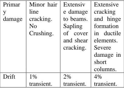
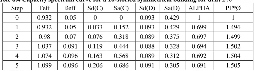
Storey drift is the displacement of one level relative to the other level above and below. Figure 6.1 and 6.2 shows the comparison of curves with and without shear wall.

From figure 6.1 and 6.2 observed that storey drift increases as the height of storey increases. The storey drifts for 10 & 15 storied building gives maximum envelop for 7, 8 storey and 10, 11 storey.

Table 6.9 Storey drifts of various storey levels

Storey level Storey drifts without shear

wall

Storey drifts with shear wall

Terrace 13.22 3.936

Storey 9 14.66 4.059

Storey 8 14.98 4.128

Storey 7 14.92 4.125

Storey 6 14.8 4.023

(9)

Storey 5 13.4 3.81

Storey 4 12.6 3.468

Storey 3 12.8 2.988

Storey 2 11.27 2.349

Storey 1 1.027 1.563

Ground level 1.250 0.726

Figure 6.1 Drifts of 10-storied building in x-direction

Table 6.10 Drifts of various storey levels

Storey level

Storey drifts without shear wall

Storey drifts with shear wall

Terrace 14.41 5.421

Storey 14 14.62 5.568

Storey 13 15.33 5.763

Storey 12 15.45 5.763

Storey 11 15.23 5.811

Storey 10 15.21 5.802

Storey 9 14.8 5.727

Storey 8 14.46 5.562

Storey 7 14.56 5.34

Storey 6 14.22 5.01

Storey 5 13.53 4.581

Storey 4 13.42 4.044

Storey 3 13.22 3.393

Storey 2 13.02 2.61

Storey 1 1.22 1.695

Figure 6.2 Drifts of 15-storied building in x-direction

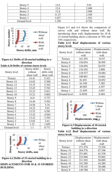
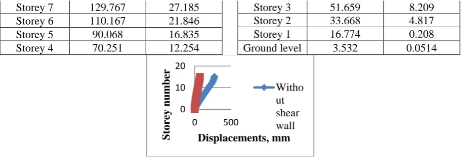
DISPLACEMENTS FOR 10 & 15 STORIED BUILDING

Figure 6.3 and 6.4 shows the comparison of curves with and without shear wall. By introducing shear wall, displacements for 10 & 15 storied building shows a decrease in 78% and 74% respectively.

Table 6.11 Roof displacements of various storey levels

Storey level

Displacements without shear

wall

Displacements with shear

wall

Terrace 161.295 34.93

Storey 9 156.054 30.995

Storey 8 146.856 26.935

Storey 7 134.102 2.808

Storey 6 118.537 18.684

Storey 5 100.861 14.661

Storey 4 81.691 10.852

Storey 3 61.549 7.385

Storey 2 40.983 4.397

Storey 1 21.859 2.047

Figure 6.3 Displacements of 10-storied building in x-direction

Table 6.12 Roof displacements of various storey levels

Storey level

Displacements without shear

wall

Displacements with shear

wall

Terrace 271.576 72.526

Storey 14 264.576 67.106

Storey 13 251.881 61.538

Storey 12 233.966 55.862

Storey 11 211.593 50.099

Storey 10 191.289 44.289

Storey 9 170.145 38.488

Storey 8 149.788 32.761

0 2 4 6 8 10 12

0 10 20

Sto

rey nu

mber

Storey drifts, mm

Without shear wall

With shear wall

0 10 20

0 20

Sto

rey nu

mber

Storey drifts, mm Witho ut shear wall

0 5 10 15

0 200

Sto

rey nu

mber

Displacements, mm Withou t shear wall

(10)

Storey 7 129.767 27.185

Storey 6 110.167 21.846

Storey 5 90.068 16.835

Storey 4 70.251 12.254

Storey 3 51.659 8.209

Storey 2 33.668 4.817

Storey 1 16.774 0.208

Figure 6.4 Displacements of 15-storeied building in x-direction

CONCLUSIONS

 When a 10 and 15 storied buildings are

pushed to 1% transient drift

(0.32m,0.47m), the performance of the

building lies between Immediate

Occupancy and Life Safety levels even with increase in the storey height. In the present case study, both the buildings have moderate resistance.

 The drift index of 10 and 15 storied buildings are 0.00406 and 0.00415 which is below the permissible index value of 0.005(for no damage as per ATC-40). It infers that the lateral displacement of the structure is well within permissible limits and no damage occurs as a whole.

 When a 10 and 15 storied buildings are

pushed to 2% transient

drift(0.64m,0.94m), the performance of the building lies between Life Safety and Collapse Prevention levels even with increase in the storey height. In the present case study, both the buildings have poor resistance.

 The drift index of 10 and 15 storied buildings are 0.00445 and 0.00459 which is below the permissible index value of 0.005(for no damage as per ATC-40). It infers that the lateral displacement of the structure is well within permissible limits and no damage occurs as a whole.

 The observed displacements at terrace level for a 10 storied building without shear wall were 161mm. When shear wall

was introduced to the structure

displacement was drastically reduced to 34.9mm. It infers that the structure is well within permissible limits and no damage occurs as a whole.

 The observed displacements at terrace level for a 15 storied building without shear wall were 271mm. When shear wall

was introduced to the structure

displacement was drastically reduced to 72.5mm. It infers that the structure is well within permissible limits and no damage occurs as a whole.

 REFERENCES

1. Habibullah and Stephen Pyle (1998), “Practical Three Dimensional Nonlinear Static Pushover Analysis”, Published in Structure Magazine, winter.

2. Kadid A and Boumrkik A (2008), “Pushover Analysis of Reinforced Concrete Framed Structures”, At

Department of civil Engineering,

University of Banta, Algeria, Asian journal of civil engineering Vol. 9(1),pp. 75-83.

3. Monavari B, Massumi A, Kazem A (2008), “Estimation of Displacement Demand in RC Frames and Comparing with Target Displacement” Provided by FEMA-356, 15th World Conference on Earthquake Engineering, 24th to 28th, Lisbon, Portugal.

4. Onur Merter and Taner Ucar (2010), “A Comparative Study on Nonlinear Static and Dynamic Analysis of Frame Structures”, Journal of civil Engineering and Science, Vol. 2(3), pp. 155-162. 5. Sudipta Chattopadhyaya and Alman K

Sengupta (2011), “Modeling of Tall Shear Walls for Non-linear Analysis of RC Buildings under Cyclic Lateral Loading”, The Indian Concrete journal, Vol. 85( 8), pp. 38-40.

0 10 20

0 500

Storey numbe

r

(11)

Available online: https://edupediapublications.org/journals/index.php/IJR/ P a g e | 2765 6. Mitchalis Fragiadakis, Dimitrios

Vamvatsikos, Mark Ascheim (2011), “Application for Seismic Assessment of Regular RC Moment Frame Buildings", Department of Civil and Environmental Engineering, University of Cyprus. Vol. 5(4), pp. 20-29.

7. A. Cinitha, P.K. Umesha, Nagesh R. Iyer (2011), “Non linear Static Analysis to Assess Performance and vulnerability of Code- Conferring RC buildings”, wseas transactions on applied and theoretical mechanics, Vol.7(1), pp. 39-48.

8. S.I. Khan and P.O. Modani (2012), “Seismic Evaluation and Retrofitting of RC Building by Using Energy Dissipating Devices”, International Journal of Engineering research and Applications, Vol. 3(3), pp. 1504-1514.

9. Chopra, A.K and Rakesh K.G (2012),

“Capacity-Demand-Diagram Methods

Based on Inelastic Design Spectrum”, Earthquake Spectra, Vol. 5(4), pp. 45-52. 10. Satpute S.G and Kulkarni D. B (2013),

“Comparative Study of Reinforced Concrete Shear Wall Analysis in Multi Storied Building with Openings by Nonlinear Methods”, International Journal of Structural and civil Engineering Research, Vol. 2(3), pp. 183-193.

11. S. Chandrasekaran and Varun Gupta (2013), “Performance Based Design for RC Framed Buildings”, Department of

Civil Engineering, Institute of

Technology, BHU.

12. Sudipta Chattopadhyaya and Amlan K. Sengupta (2014), “Modeling of Tall Shear

walls for pushover analysis of reinforced concrete buildings”, The Indian Concrete Journal Vol. 8(4), pp. 7-13.

13. Mwafy A. M. and Elnashai A. S (2014), “Static Pushover versus Dynamic Analysis of RC Buildings”, Engineering Structures, Vol. 23, pp. 407-424.

14. N. Lakshmanan (2014), “Seismic Evaluation and Retrofit of Buildings and Structures”, ISET Journal of Earthquake Technology, Vol. 43(2), pp. 31-48.

15. Tamboli H. R. and Karadi U. N (2014), “Seismic Analysis of RC Frame Structure with and without Masonry Infill Walls”, Indian Journal of Natural Sciences”, Vol. 3(14), pp. 138-144.

16. FEMA 440 (2005), “Guidelines For improvement of non-linear static seismic analysis procedure”.

17. ATC 40 (1996), “Seismic Evaluation and Retrofit of Concrete Buildings”, vol.1, Applied technology council, Redwood city, CA.

18. FEMA 356 (2000), “Pre standard and Commentary for the Seismic Rehabilitation of Buildings”, American Society of Civil Engineers, Reston, VA. 19. IS 1893 (2002), Indian Standard-

“Criteria for Earthquake Resistant Design of Structures”, General provisions and buildings (fifth revision).