Ludwig-Maximilians-Universität
Sigillum Universitatis Ludovici Maximiliani
Bayesian Methods for Analyzing the Large Scale
Structure of the Universe
Dissertation an der Fakultät für Physik
der Ludwig-Maximilians-Universität München
für den Grad des
Doctor rerum naturalium
vorgelegt von Jens Jasche
aus Essen
Dissertation der Fakultät für Physik der Ludwig-Maximilians Universität München
ausgeführt am Max-Planck-Institut für Astrophysik
"We take o
ff
into the cosmos, ready for anything: for solitude, for hardship, for
exhaustion, death. Modesty forbids us to say so, but there are times when we think
pretty well of ourselves. And yet, if we examine it more closely, our enthusiasm
turns out to be all a sham. We don’t want to conquer the cosmos, we simply want
to extend the boundaries of Earth to the frontiers of the cosmos. For us, such and
such a planet is as arid as the Sahara, another as frozen as the North Pole, yet
another as lush as the Amazon basin. We are humanitarian and chivalrous; we don’t
want to enslave other races, we simply want to bequeath them our values and take
over their heritage in exchange. We think of ourselves as the Knights of the Holy
Contact. This is another lie. We are only seeking Man. We have no need of other
worlds. A single world, our own, su
ffi
ces us; but we can’t accept it for what it is.
We are searching for an ideal image of our own world: we go in quest of a planet,
a civilization superior to our own but developed on the basis of a prototype of our
primeval past. At the same time, there is something inside us which we don’t like to
face up to, from which we try to protect ourselves, but which nevertheless remains,
since we don’t leave Earth in a state of primal innocence. We arrive here as we are in
reality, and when the page is turned and that reality is revealed to us - that part of our
reality which we would prefer to pass over in silence - then we don’t like it anymore."
Contents
1. Abstract 1
2. Introduction and motivation 5
2.0.1.
Motivation
. . . .
5
2.0.2.
Structure
. . . .
7
3. Cosmology and cosmic structure formation 9
3.1. Friedmann-Lemaître cosmological models
. . . .
9
3.1.1.
A general relativistic universe
. . . .
9
3.1.2.
Cosmological principles and the Robertson-Walker metric
. . . .
10
3.1.3.
Friedmann world model
. . . .
12
3.1.4.
Distance measures in cosmology
. . . .
13
3.2. Structure formation
. . . .
14
3.2.1.
Growth of density perturbations in cold dark matter models
. . . .
15
3.2.2.
Zel’dovich approximation
. . . .
19
3.2.3.
Numerical simulations of cosmic structure formation
. . . .
20
3.3. Large scale structure
. . . .
20
3.3.1.
Distribution of matter in the Universe
. . . .
20
3.3.2.
Statistical description of the large scale structure: Gaussian random fields
. . . .
22
3.3.3.
Statistical description of the large scale structure: Lognormal random fields
. . .
24
4. The Sloan Digital Sky Survey 27
4.1. Introduction to the Sloan Digital Sky Survey
. . . .
27
4.1.1.
SDSS surveys
. . . .
27
4.1.2.
Instrument description
. . . .
28
4.1.3.
Acknowledgement
. . . .
28
5. Data processing 31
5.1. Introduction
. . . .
31
5.2. The requirements of FFTs
. . . .
34
5.3. Discretizing the real-space
. . . .
34
5.3.1.
Sampling theorem
. . . .
34
5.3.2.
Low-Pass-Filtering
. . . .
36
5.3.3.
Sampling on a finite real-space domain
. . . .
37
5.4. Discretizing The Fourier-space
. . . .
38
5.4.1.
FFTs and the Fourier-space representation
. . . .
38
5.4.2.
Sampling in Fourier-space
. . . .
40
5.4.3.
The instrument response function of our computer and the loss of information
. .
42
5.5. Sampling 3d galaxy distributions
. . . .
43
5.5.1.
Ideal sampling procedure
. . . .
43
5.6.1.
Filter approximation
. . . .
45
5.7. Supersampling
. . . .
46
5.7.1.
Super resolution and downsampling
. . . .
47
5.8. Discussion and conclusion
. . . .
48
6. Bayesian inference 53
6.1. Introduction
. . . .
53
6.2. Conventional vs. Bayesian statistics
. . . .
54
6.3. Conditional probabilities
. . . .
55
6.4. The prior distribution and the mechanism of empirical learning
. . . .
56
6.5. Markov Chain Monte Carlo methods
. . . .
58
6.5.1.
The Monte Carlo principle
. . . .
58
6.5.2.
Markov Chain Monte Carlo algorithms
. . . .
59
6.5.3.
Metropolis-Hastings algorithm
. . . .
60
6.5.4.
Gibbs sampling
. . . .
61
6.6. Summary
. . . .
62
7. ARES - Joint inference of the three dimensional density field and its power-spectrum 63
7.1. Introduction
. . . .
63
7.2. Notation
. . . .
65
7.3. The Large scale structure Gibbs sampler
. . . .
66
7.3.1.
Gibbs sampling
. . . .
66
7.3.2.
Joint power-spectrum and density field inference
. . . .
67
7.4. Sampling the signal maps
. . . .
68
7.4.1.
The Wiener filter
. . . .
68
7.4.2.
The galaxy data model
. . . .
70
7.4.3.
Drawing signal samples
. . . .
73
7.5. Sampling the power-spectrum
. . . .
75
7.5.1.
Drawing power-spectrum samples
. . . .
75
7.5.2.
Blackwell-Rao estimator
. . . .
78
7.6. The prior and the cosmic variance
. . . .
79
7.6.1.
Flat versus Je
ff
reys’ prior
. . . .
79
7.6.2.
Informative prior
. . . .
80
7.6.3.
Hidden prior
. . . .
81
7.7. Numerical Implementation
. . . .
83
7.7.1.
Inversion of matrices
. . . .
85
7.7.2.
Random number generation
. . . .
85
7.7.3.
Parallelization
. . . .
85
7.8. Testing ARES
. . . .
87
7.8.1.
Setting up a Gaussian Mock observation
. . . .
87
7.8.2.
Testing convergence and correlations
. . . .
87
7.8.3.
High resolution Simulation
. . . .
91
7.8.4.
Testing an informative Prior
. . . .
92
7.8.5.
Testing with galaxy mock catalogs
. . . .
93
7.9. Operations on the set of Gibbs samples
. . . .
94
Contents
8. HADES - A fast Hamiltonian sampler for large scale structure inference 99
8.1. Introduction: non-linear sampling
. . . .
99
8.2. The lognormal distribution of density
. . . .
100
8.3. Lognormal Poissonian posterior
. . . .
101
8.4. Hamiltonian sampling
. . . .
102
8.5. Equations of motion for a log-normal Poissonian system
. . . .
103
8.6. Numerical Implementation
. . . .
104
8.6.1.
The leapfrog scheme
. . . .
105
8.6.2.
Hamiltonian mass
. . . .
105
8.6.3.
Parallelization
. . . .
105
8.7. Testing HADES
. . . .
106
8.7.1.
Setting up Mock observations
. . . .
106
8.7.2.
Burn in behavior
. . . .
108
8.7.3.
Convergence
. . . .
110
8.7.4.
Testing with simulated galaxy surveys
. . . .
111
8.8. Summary and Conclusion
. . . .
111
9. Nonlinear density field inference from SDSS data 115
9.1. Introduction
. . . .
115
9.2. Classification of the cosmic web
. . . .
117
9.3. DATA
. . . .
119
9.3.1.
The SDSS galaxy sample
. . . .
119
9.3.2.
Completeness and selection function
. . . .
120
9.3.3.
Creating the three dimensional data cube
. . . .
120
9.3.4.
Physical model
. . . .
122
9.4. Results
. . . .
123
9.4.1.
Convergence test
. . . .
124
9.4.2.
Hamiltonian samples
. . . .
124
9.4.3.
Ensemble mean and variance
. . . .
124
9.5. Web classification
. . . .
126
9.6. Galaxy properties versus LSS
. . . .
127
9.7. Summary and Conclusion
. . . .
129
10. Summary and outlook 135 A. APPENDIX 139
A.1. Continuous Fourier transformation
. . . .
139
A.1.1. Convolution Theorem
. . . .
139
A.1.2. Fourier transform of the sampling operator
. . . .
140
A.1.3. Fourier transform pair of the ideal low pass filter
. . . .
140
A.1.4. Fourier transform of the finite sum sampling operator
. . . .
141
A.1.5. Ideal discretization kernel
. . . .
141
A.1.6. Discrete Fourier transformation
. . . .
142
A.1.7. Discrete mode coupling function
. . . .
143
A.2. Change to FFT representation
. . . .
144
A.3. Wiener Variance
. . . .
146
A.4. Hamiltonian Masses
. . . .
147
1. Abstract
Bayesian methods for Large Scale Structure analysis
The cosmic large scale structure is of special relevance for testing current cosmological theories about the
origin and evolution of the Universe. Throughout cosmic history, it evolved from tiny quantum
fluctua-tions, generated during the early epoch of inflation, to the filamentary cosmic web presently observed by
our telescopes. Observations and analyses of this large scale structure will hence test this picture, and will
provide valuable information on the processes of cosmic structure formation as well as they will reveal
the cosmological parameters governing the dynamics of the Universe.
Beside measurements of the cosmic microwave backround, galaxy observations are of particular interest
to modern precision cosmology. They are complementary to many other sources of information, such as
cosmic microwave background experiments, since they probe a di
ff
erent epoch. Galaxies report the
cos-mic evolution over an enormous period ranging from the end of the epoch of reionization, when luminous
objects first appeared, till today. For this reason, galaxy surveys are excellent probes of the dynamics and
evolution of the Universe. Especially the Sloan Digital Sky Survey is one of the most ambitious surveys
in the history of astronomy. It provides measurements of 930,000 galaxy spectra as well as the according
angular and redshift positions of galaxies over an area which covers more than a quarter of the sky. This
enormous amount of precise data allows for an unprecedented access to the three dimensional cosmic
matter distribution and its evolution. However, observables, such as positions and properties of galaxies,
provide only an inaccurate picture of the cosmic large scale structure due to a variety of statistical and
systematic observational uncertainties. In particular, the continuous cosmic density field is only traced
by a set of discrete galaxies introducing statistical uncertainties in the form of Poisson distributed noise.
Further, galaxy surveys are subject to a variety of complications such as instrumental limitations or the
nature of the observation itself. The solution to the underlying problem of characterizing the large scale
structure in the Universe therefore requires a statistical approach.
into the non-linear regime. In particular, HADES accurately treats the non-linear relationship between
the observed galaxy distribution and the underlying continuous density field by correctly accounting for
the Poissonian nature of the observables. This allows for very precise recovery of the density field even
in sparsely sampled regions. HADES also provides a complete statistical description of the non-linear
cosmic density field in the form of a sampled representation of a cosmic density posterior. Beside the
possibility of reporting any desired statistical summary of the density field or power-spectrum, such
rep-resentations of the according posterior distributions also allow for simple non-linear and non-Gaussian
error propagation to any quantity finally inferred from the analysis results. The application of HADES to
the latest Sloan Digital Sky Survey data denotes the first fully Bayesian non-linear density inference
con-ducted so far. The results obtained from this procedure represent the filamentary structure of our cosmic
neighborhood in unprecedented accuracy.
Bayesische Methoden zur Analyse der großskaligen Struktur
Die großskalige Struktur der kosmischen Materieverteilung ist von besonderer Bedeutung für die
Über-prüfung moderner kosmologischer Modelle des Ursprungs und der weiteren Entwicklung des Universums.
Im Verlauf der kosmischen Geschichte hat sich diese Struktur aus mikroskopischen Quantenfluktuation,
welche zur Epoche der Inflation erzeugt wurden, zu dem heute mittels Teleskopen beobachteten
faser-förmigen kosmischen Netz entwickelt. Beobachtungen und Analysen dieser großskalige Struktur prüfen
daher dieses Bild, und liefern wertvolle Information über die Prozesse der kosmologischen
Strukturbil-dung als auch über die kosmologischen Parameter, welche die Dynamik des Universums bestimmen.
Neben Messungen des kosmischen Mikrowellenhintergrundes, sind insbesondere
Galaxienbeobachtun-gen von großem Interesse für die moderne Präzisionskosmologie. Sie ergänzen viele andere
Informa-tionsquellen, wie den Mikrowellenhintergrund, da sie Aufschluss über verschiedene kosmische Epochen
geben. Galaxien verfolgen die kosmische Entwicklung über enorme Zeiträume, ausgehend vom Ende
der Reionisationsepoche, als die ersten leuchtenenden Objekte entstanden, bis heute. Daher sind
Galax-ienbeobachtungen besonders geeignet die Dynamik und Entwicklung unseres Universums zu studieren.
Insbesondere der Sloan Digital Sky Survey ist eines der ambitioniertesten Galaxienbeobachtungsprojekte
in der Geschichte der Astronomie. In diesem Projekt wurden Spektren von 930.000 Galaxien, so wie
deren Winkelpositionen und Rotverschiebungen, in einer Fläche erfasst, welche mehr als ein Viertel des
Himmels abdeckt. Diese enorme Datenmenge ermöglicht einen noch nie dagewesenen Zugang zu der
dreidimensionalen kosmischen Materieverteilung und deren Entwicklung. Jedoch liefern
Beobachtungs-grössen, wie die Positionen und Eigenschaften der Galaxien, wegen einer Vielzahl von statistischen und
systematischen Beobachtungsunsicherheiten, nur ein ungenaues Bild der großskaligen Struktur im
Uni-versum. Insbesondere wird das kontinuierliche kosmische Dichtefeld nur durch eine Menge von diskreten
Galaxien nachgezeichnet, was statistische Unsicherheiten in der Form von poisson-verteiltem Rauschen
erzeugt. Des Weiteren unterliegen Galaxienbeobachtungen einer Menge von zusätzlichen
Komplikatio-nen, wie instrumentelle Limitierungen oder der intrinsischen Natur der Beobachtung selbst. Die Lösung
des unterliegenden Problems, der Charakterisierung der großskaligen Struktur im Universum, bedarf
da-her im Allgemeinen eines statistischen Ansatzes.
2. Introduction and motivation
2.0.1. Motivation
The subject of cosmology has always been amongst the prime interests of humanity, since it tries to
de-scribe and explain the origin and the properties of the Universe and eventually the existence of man. While
originally being defined by religious or philosophical ideology, over the past centuries natural sciences
started to govern our modern view of the Universe. Particularly within the last century great advancements
have been made, elevating the subject of cosmology from a mere philosophical to an accurate scientific
discipline. Physics and Astrophysics hereby played the crucial role in shaping the understanding of the
Universe by establishing a scientific theory about its origin and evolution. The foundations of modern
cosmological models have been laid by the early discovery of E. Hubble and the development of general
relativity by A. Einstein. Hubble observed that the recession velocities of galaxies are proportional to their
distances, indicating that spacetime itself is not static, as expected from Newtonian theories, but
expand-ing. This observation induced the development of relativistic cosmological models based on solutions of
Friedmann’s equations by A. Einstein and W. de Sitter. These solutions describe an expanding universe
suggesting that it must have originated from a much hotter and denser state as can be observed today. The
idea of a hot Big Bang as the origin of the Universe was further shaped by theoretical investigations of
R. Alpher, H. Bethe and G. Gamov. They studied the thermal history of an expanding universe and found
that at early times it was hot and dense enough to allow for thermonuclear synthesis of light elements.
Support for their theory was given by measurements of the cosmic abundance of light elements, in
partic-ular of deuterium. Their theory further predicted the existence of a cosmic microwave background, which
was subsequently detected by A. A. Penzias and R. W. Wilson.
In the course of the last and the beginning of this century, cosmologists have constrained the parameters
governing the homogeneous dynamics of the Universe, as described by Friedmann’s equations, to the few
percent level and cosmology turned to investigating the cosmic inhomogeneities.
According to the current cosmological paradigm, all observed structures have their origin in microscopic
primordial quantum fluctuations generated during the first split seconds of the Universe. I. Novikov and
Y .B. Zel’dovich suggested that over the following 13.6 billion years, these tiny seed perturbations formed
the presently observed matter distribution via gravitational amplification. J. Peebles then realized that
baryonic models of structure formation are insu
ffi
cient to explain observations and introduced a new not
electromagnetically interacting matter component. Therefore, currently it is believed that structure
forma-tion is governed by the gravitaforma-tional aggregaforma-tion of such a dark matter fluid. As proposed by J. P. Ostriker,
M. Rees and S. D. M. White, luminous objects like galaxies then form inside dark matter structures by
condensation and cooling of baryons.
The process of structure formation hence involves very exciting physics ranging from quantum field
theory, general relativity to the dynamics of collisionless dark matter and the behavior of the baryonic
sector. Throughout cosmic history, these processes imprinted a wealth of information on the origin and
evolution of the Universe to the large scale matter distribution as we observe it today. Thus, observations
of the cosmic large scale structure have the potential to answer many open questions in physics and
cosmology, such as:
•
Is dark matter hot or cold?
•
What is the dynamical behavior of our Universe?
•
How is matter distributed?
•
Does dark energy exist and how does it behave?
•
Is our model of gravity correct or does it require modification?
•
How do galaxies form, and how are they tracing dark matter?
•
What were the conditions in the early Universe?
Harvesting this information from present and future probes of the large scale structure, such as galaxy
surveys or cosmic microwave background experiments hence allows for testing current physical and
cos-mological theories. Especially, the large scale distribution of galaxies provides information about the
clustering of dark matter on small scales and the transition from linear to nonlinear structure formation.
Theories of cosmological structure formation are usually tested by determining the statistical properties
of the dark matter density field or any tracer of it, like the galaxy distribution. In particular, statistical
characterization in terms of power-spectra or
n
-point correlation functions has become a major method
for large scale structure analyses over the past decades. Precise determination of the overall shape of
the power-spectrum can for instance place important constraints on neutrino masses, help to identify the
primordial power-spectrum and break degeneracies for cosmological parameter estimation from cosmic
microwave background data by measuring the parameter combination
Ω
m/
h
. In addition, several
char-acteristic length scales have been imprinted to the matter distribution, which can serve as new standard
rulers to measure the Universe. A prominent example of these length scales is the sound horizon, which
yields oscillatory features in the power-spectrum, the so-called baryon acoustic oscillations. Such a new,
precise standard ruler will enable us to measure the Universe through the distance redshift relation and
to test various dark energy scenarios. The aim of all these observations is to determine the cosmological
parameters governing the cosmological structure formation to a degree of accuracy comparable to those
governing the homogeneous dynamics of the Universe. Beside direct observations, theories of structure
formation are investigated with numerical computer simulations. These computer simulations solve the
equations of motion for the matter content in the Universe and provide insight into dark matter dynamics
in the nonlinear stages of structure formation and baryonic physics in the core of galaxies and clusters of
galaxies.
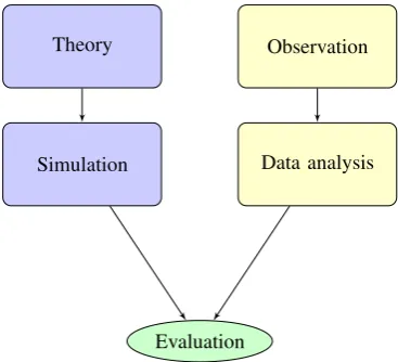
2.0.2 Structure
Figure 2.1.: The scientific progress in natural sciences depends on the four steps of theoretical modelling, simulations, observations and data analysis. The results of simulations and data analysis can be compared to judge and evaluate current models.
reality, and each measurement is subject to a variety of uncertainties. A following data analysis procedure
must abstract the signal one seeks to recover from those uncertainties and must also provide a measure
of confidence in the obtained result. The agreement of the theoretical prediction and the result of the
data analysis can then be compared within the confidential limits, and only then a theory can be evaluated
or judged to be plausible or not. This demonstrates the importance of data analysis procedures for any
natural science including cosmology.
This thesis is dedicated to the development of new Bayesian methods to perform joint inferences of
full three dimensional density fields and their power-spectra from cosmological data sets, especially from
galaxy redshift surveys. In particular, the developed computer algorithms are designed to correct
obser-vational systematics, such as survey geometries and selection e
ff
ects, and statistical uncertainties, such as
noise and cosmic variance. Based on very e
ffi
cient Markov Chain Monte Carlo algorithms, required to
explore extremely high dimensional parameter spaces, these algorithms provide sampled representations
of the according posterior distributions conditional on galaxy observations. These posterior distributions
contain the full joint information on the signal one seeks to recover and its uncertainties. Any desired
statistical summary can easily reported and theoretical models can be estimated via Bayesian model
com-parison. The data analysis methods as presented in this thesis provide a full statistical characterization
of the observed large scale structure and its uncertainties as well as a sound cosmographic description in
the form of three dimensional maps of the cosmic density field. Results obtained from the applications
of these methods to the latest Sloan Digital Sky Survey data, therefore allow for precise studies of the
cosmological structure formation, the correlation of galaxy properties and the large scale structure as well
as for the analysis of the cosmological parameters governing the dynamics of the Universe.
2.0.2. Structure
to unprecedented details.
Chapter
5
is more technical in nature. Here the basic concepts of data acquisition and processing
with digital computers are presented. In particular, the implications of Shannon’s sampling theorem
and the application of Fast Fourier Transform techniques for information recovery from sampled data
systems are discussed to great detail. Further, a super sampling method is presented which can greately
alleviate sampling artifacts, such as aliasing, in power-spectrum estimations. It is particularly designed for
iterative data analysis methods, such as Wiener filtering, in which artificial mode coupling, as introduced
by systematic observational e
ff
ects, is to be corrected correctly.
In Chapter
6, basic epistemological concepts and the mathematical framework of Bayesian statistics
and statistical data analysis are presented. A brief overview of frequently encountered statistical and
systematic uncertainties in galaxy redshift surveys and a motivation for the requirement of statistical
data analysis is provided. Further, Bayesian and conventional statistics are compared and di
ff
erences,
particularly concerning the notion of probability, are highlighted. Then key concepts of Markov Chain
Monte Carlo techniques will be presented and discussed to a degree required for this thesis.
Chapter
7
describes the development and implementation of the Bayesian data analysis computer
al-gorithm ARES (Alal-gorithm for REconstruction and sampling). This alal-gorithm aims at the joint inference
of three dimensional density fields and power-spectra from a given cosmological data set by exploring
the joint posterior distribution via an e
ffi
cient Gibbs sampling scheme. In this fashion, ARES provides
a sampled representation of the joint posterior distribution from which any desired statistical summary,
such as mean, mode or variance, can be easily reported. Mock tests demonstrate the ability of ARES to
recover the power-spectra from observations with highly structured survey geometries, selection e
ff
ects
and noise to great accuracy. In particular, the problem of artificial mode coupling can be accounted for
correctly yielding a high detectability of the baryon acoustic oscillations in the inferred power-spectrum.
In Chapter
8, a new method for non-linear three dimensional density field inference is presented. The
resultant computer algorithm HADES (HAmiltonian Density Estimation and Sampling), provides samples
from a lognormal Poissonian posterior via an e
ffi
cient hybrid Hamiltonian Monte Carlo sampler. The
method is tested in various mock scenarios, which demonstrate the ability of HADES to recover the fully
evolved non-linear density field to great accuracy.
Chapter
9
presents the application of the non-linear sampler HADES to the latest Sloan Digital Sky
Survey data. This procedure yields a sampled representation of the three dimensional density posterior
conditional on galaxy observations. The estimated ensemble mean density field reveals the filamentary
cosmic-web as predicted by numerical simulations. Further, a dynamical cosmic web type analysis is
conducted to identify the four di
ff
erent structure types halos, filaments, sheets and voids. A preliminary
analysis of correlations between galaxy properties and large scale environment is also provided.
3. Cosmology and cosmic structure formation
Abstract
This chapter provides an overview of the current cosmological theory and the process of cosmic structure formation as relevant for this thesis. In Sect.3.1key concepts of general relativistic Friedmann-Lemaître cosmological models will be discussed, followed by the presentation of the theory of cosmological structure formation in Sect.3.2and the description of the statistical properties of the large-scale structure is presented in Sect.3.3.
3.1. Friedmann-Lemaître cosmological models
The overall evolution of the Universe from the beginning to its present state is generally governed by gravitational interactions. For this reason, modern cosmological world models are based on the theory of general relativity, as presented by A. Einstein in 1915 (Einstein 1915). Einstein’s theory describes gravity as an emergent geometric property of space and time. In the following, a brief overview over the foundations of modern cosmological world models is given.
3.1.1. A general relativistic universe
In general relativity spacetime is a four-dimensional manifold described by a metric tensor gµ ν, which defines the geometric relation between two spacetime events. Such spacetime events are given by their four dimensional world coordinates, described by four-vectorsxµcontaining the time coordinates and three spatial coordinates. Any infinitesimal separation dsbetween these events, separated by dxµ, can then be calculated with the metric tensor by ds = gµ νdxµdxν. Here we used Einstein summation convention, which means to sum over repeated indices. According to general relativity the components of the metric tensorgµ νare the dynamical variables which generate the gravitational interaction.
A cosmological world model hence requires to describe the dynamical behavior of the metric tensor along with that of the material and energetic contents of the Universe. The dynamics of such a model can be derived from a generalized Einstein-Hilbert action (see e.g.Gibbons & Hawking 1977,Carroll 2004):
S =
Z
d4x√−gL=
Z
d4x√−g Lg+Lm+Lq, (3.1) whereLg,LmandLqare the Lagrange densities for the metric tensor, the matter field and a possible dark energy
component respectively. For models of Einstein gravity with a cosmological constant the sum of Lagrangians for gravity and dark energy can be written as:
Lg+Lq= c4
16πG (R−2Λ) (3.2)
where R = gµνRδµδν is the Ricci scalar, with Rδµγν being the Riemann tensor1, and Λdenotes the cosmological
constant. Variation of the Einstein-Hilbert action, given in eq. (3.1), with respect to the metric tensorgµ ν yields
then Einstein’s field equations (Landau & Lifshitz 1975,Carroll 2004):
Gµν≡Rµν−R
2gµν= 8πG
c4 Tµν+ Λgµν, (3.3)
1The Riemann tensor is defined asRδ
whereGµν is is the Einstein tensor, Rµν =Rδµδν is the Ricci tensor andTµν is the energy momentum tensor of the
matter component obtained by variation ofLmwith respect to the metric tensor (see e.g.Gibbons & Hawking 1977,
Carroll 2004). Einstein’s equation form a set of ten independent second-order differential equations for the metric tensorgµ ν(Carroll 2004). However, the Bianchi identity∇µGµν =0, with∇µbeing the covariant derivative, provides
four constraints on the Ricci tensor which reduces the amount of equations to six truly independent equations, as is required for the metric to be a solution to Einstein’s equations in any coordinate system. Another consequence of the contracted Bianchi identity is that the energy momentum tensor is a conserved current, i.e.∇µTµν =0. The major difficulty for solving Einstein’s equations arises from the high degree of non-linearity. Hence, two known solutions can generally not be superposed to find a new one. Solutions of the Einstein’s equations therefore often require simplifying assumptions as will be discussed in the following. Also note, that the action given in eq. (3.1) is the most fundamental way to summarize our current understanding of the Universe.
3.1.2. Cosmological principles and the Robertson-Walker metric
Einstein’s equations are fundamentally governing the dynamical evolution of the Universe. Hence, any conclusive cosmological model must be based on a solution to this set of non-linear equations. Since no general solution to Einstein’s equations is known, one usually has to be content with an ansatz for the metric tensor. In order to further reduce the number of coupled equations to solve, one usually requires metric tensor to be highly symmetric. Such an ansatz for the metric in a cosmological model can be found by requiring the metric to fulfill the cosmological principles, as stated below.
3.1.2.1. The cosmological principles
In modern standard cosmological theories, Einstein’s equations are commonly solved by assuming a spherically symmetric metric tensorgµ ν, which describes the expansion dynamics of the Universe. This simplifying assumption
for the cosmological model is based on two fundamental postulates.
• Isotropy:
When averaged over sufficiently large scales, there exists a mean motion of matter and radiation in the Universe. For an observer co-moving with such mean motion, all averaged observables appear to be isotropic.
• Homogeneity:
There exists no preferred position for any observer following this mean motion. Thus, all observers mea-sure the same averaged observables and experience the same history of the Universe (also known as the Copernican principle (Peacock 1999)).
These postulates reflect our believe that the large scale universe is homogeneous and isotropic. Throughout most of the twentieth century, when the foundations for modern cosmology were developed, in particular by Friedmann and Lemaître, the cosmological principles were an educated guess to solve Einstein’s equations. Today firm empirical data exists, confirming the large scale homogeneity and isotropy of the Universe (Mukhanov 2005). Support for the first postulate is given by the observation of perfect rotational invariance of the cosmic microwave background (CMB) temperature in the co-moving frame. By assuming the isotropy of the spatial hyper-surface around any such co-moving observer and applying the cosmological principle in space yields isotropy around any point on the spatial hyper-surface. Given the space-time metric is an analytic function of the coordinates, this immediately implies homogeneity. The observable region of the Universe is on the order of 3 Gpc, and modern galaxy redshift surveys suggest that the Universe is only homogeneous and isotropic when averaged on scales& 100 Mpc. On smaller scales the Universe is highly inhomogeneous, filled with aggregations of matter, such as galaxies, clusters and superclusters (Mukhanov 2005). Therefore, the cosmological principle is only applicable within a limited range of scales.
3.1.2.2. The Robertson-Walker metric
3.1.2 Cosmological principles and the Robertson-Walker metric
deduced from a coordinate system xµin the reference frame of such a fundamental observer. Then the spacetime interval ds2can be separated out (Padmanabhan 1993):
ds2=gµνdxµdxν=g00c2dt2+2g0icdtdxi+gi jdxidxj, (3.4)
where Latin indices denote summations only over the spatial components. In the reference frame of a fundamental observer one may use the proper time of such an observer to label the spatial hyper-surfaces, which impliesg00 =1.
Further, if the metric tensor is to fulfill the requirement of isotropy the componentsgi0must vanish, since otherwise
a particular direction in space is preferred. Thus, a metric which satisfies the cosmological principles yields a line element of the form:
ds2= c2dt2+gi jdxidxj, (3.5)
Since isotropy has to be conserved, the spatial part of the metric tensor may only scale with a functiona(t) depending solely on the proper cosmic timet, yielding the line element:
ds2 =c2dt2−a2(t)dq2, (3.6) where dqis the line element on the spatial hyper-surfaces. The Robertson-Walker line element for a homogeneous and isotropic universe is then obtained by introducing spherical coordinates q = (w, θ, φ) (Misner et al. 1973,
d’Inverno 1992):
ds2=c2dt2−a2(t)hdw2+fK2(w)dθ2+sin2θdφ2i. (3.7) Due to the requirement of homogeneity the function fK(w) has to be either trigonometric for positive values of the curvatureK, linear for vanishingKor hyperbolic for negativeK:
fK(w)=
1 √ Ksin √
Kw ,(K>0), spherical,
w ,(K=0), flat,
1
√ |K|sinh
√
|K|w,(K<0), hyperbolic.
(3.8)
As one can see the highly symmetric Robertson-Walker metric is completely determined by two parameters, the curvatureKand the cosmic scale factora(t). The curvature parameterKdistinguishes between different geometries for the spatial hyper-surfaces. An open universe is determined byK <0, a flat byK =0 and a closed universe by
K>0. Today it is commonly assumed that the Universe is flat or at least close to flat. The cosmological scale factor on the other hand, describes the conformal mapping between hyper-surfaces separated by time-like vectors. From a dynamical point of view this parameter describes the dynamical behavior of the Universe. Hence, the cosmic scale factor and the dependence ofKon the matter content of the Universe uniquely determine the spacetime of a homogeneous and isotropic universe.
3.1.2.3. The cosmological redshift
The expansion of the Universe, due to the cosmological scale factor, has consequences for observing distant light sources. In an expanding universe, photons of wavelengthλs emitted by a co-moving light source at timetswill
generally be observed with the redshifted wavelengthλo atto. Since photons are massless particles, they travel
on null geodesics of zero proper time, implying the relationc2dt2 =a2(t)dq2. The co-moving distanced between emitter and observer can then be calculated according to:
d=
Z d
0
dq=
Z to
ts
dt c
a(t). (3.9) Already by construction, the co-moving distance between emitter and observer is constant. For this reason, subse-quently emitted photons at the timets+λs/cwhich are observed at the timeto+λo/cwill have traveled the same
co-moving distanced. One can therefore write:
Z to
ts
dt c a(t) =
Z to+λo/c ts+λs/c
dt c
Parameter
symbol
value
Hubble parameter
h
0
.
705
±
0
.
013
1Total matter density
Ω
m0
.
27
±
0
.
04
2Baryon density
Ω
b0
.
0456
±
0
.
0015
1Cosmological constant
Ω
Λ0
.
726
±
0
.
015
1Curvature parameter
Ω
c0
.
02
±
0
.
02
21 Komatsu et al.(2009) 2 Spergel et al.(2003)
Table 3.1.:Cosmological parameters.
If the cosmic scale factora(t) is approximately constant over the small time intervalsλs/candλo/cthen eq. (3.10)
yields the relation:
λo
λs = a(to)
a(ts) ≡1+z, (3.11) where 1+zis the relative change in wavelength, andzis referred to as the cosmological redshift. Note that this redshift is not the same as the conventional Doppler effect in special relativity, since it is due to the expansion of space itself, not to the relative velocities of the observer and emitter (Carroll 2004).
3.1.3. Friedmann world model
To study the average dynamical behavior of the Universe, Friedmann proposed a solution to Einstein’s equations, which describe an expanding homogeneous and isotropic universe (Friedmann 1922,1924). This model can be derived by assuming the contents of the Universe to behave as a homogeneous perfect fluid. The energy momentum tensor of such a fluid is completely determined by the energy densityρ, the pressurepand its four velocityuµ:
Tµν =
ρ+ p c2
uµuν−pgµν (3.12)
Together with the Robertson-Walker ansatz for the metric tensorgµν, this assumption allows for reducing the set of
Einstein’s equations given in eq. (3.3) to two ordinary differential equations: ˙
a a =
r
8πG
3 ρ−K
c2
a2 +
Λc2
3 and ¨
a a =−
4πG
3 ρ+ 3p c2
!
+Λc2
3 , (3.13) which describe the time evolution of the cosmic scale factor a(t) depending on the energy density ρ(t) and the pressurep(t) of a cosmological fluid. By virtue of the Bianchi identity∇µGµν =0, and consequently∇µTµν =0, one can further derive the adiabatic equation:
d dt
h
a3(t)c2ρ(t)i+p(t)d dta
3
(t)=0, (3.14) which describes the time evolution of the energy contained in a fixed co-moving volume expanding with the Hubble flow. Further, any change in internal energy da3(t)c2ρ(t)inside a volume is equal to the workp(t)da3(t)done
to change the proper volume. The adiabatic equation therefore corresponds to the first law of thermodynamics applied to the cosmological expansion. Alternatively this adiabatic equation can be derived by combining the two Friedmann equations (3.13). The expansion dynamics of the Universe is conveniently characterized by the Hubble functionH(t), which is defined as the logarithmic derivative of the cosmic scale factora(t):
H(t)≡ d
dtln(a)=
˙
a
a =⇒ H
2(t)=H2 0
"
8πG
3 ρ−K
c2 a2 +
Λc2
3
#
. (3.15)
3.1.4 Distance measures in cosmology
ρcrit:
ρcrit≡
3H20
8πG, (3.16)
which defines the critical point between an expanding and a contracting universe. This means, if the sum of all cosmological fluid densities givesρcrit, the curvature parameterKvanishes and all spatial hyper-surfaces are flat.
Expressing the energy densities of all cosmological fluids ( matterρ, curvatureK, the cosmological constantΛand radiation 3p/c2) in units ofρ
crit:
Ωm=
ρ ρcrit
, Ωr=
8πG p c2H2
0
, ΩΛ= Λ
3H02, Ωc= Kc2
H02 , (3.17)
allows for rewriting the Hubble function in its usual form as:
H2(t)=H02
"Ω
r a4 +
Ωm a3 −
Ωc a2 + ΩΛ
#
. (3.18)
Today, the cosmological parameters governing the homogeneous evolution of the Universe have been measured to a few percent accuracy. Particularly measurements of the CMB temperature fluctuations, as carried out by the WMAP satellite, in combination with Type Ia supernovae and baryon accoustic oscillations data, provide the most precise estimates for the set of cosmological parameters (Spergel et al. 2003,Komatsu et al. 2009). Currently, the most uncertain parameter is the value of the Hubble function at the present timeH(t0)=H0 =100hkms−1Mpc−1,
withh expressing its uncertainty. Nevertheless, measurements of CMB anisotropies and from Cepheid variable stars in distant galaxies now converge on a value ofh ' 0.7 (Freedman et al. 2001,Spergel et al. 2003,Komatsu et al. 2009). Table3.1shows the values for the cosmological parameters matter densityΩm, baryonic densityΩb,
curvatureΩc=and cosmological constantΩΛ. Since the energy density of radiation decreases rapidlyΩrdoes not
play a crucial role for the cosmological dynamics at the present epoch. One of the most important and interesting questions about the homogeneous evolution of the Universe concerns the origin and the nature of the cosmological constantΛ. Theoretical models propose that the currently observed accelerated expansion of the Universe can be explained by a new homogeneous dynamical component of the cosmological fluid the so-called dark energy, rather than by a cosmological constant. These theories suggest that the accelerated expansion of the Universe is driven by a new quantum scalar fieldφq, which exhibits negative pressure (Wetterich 1995,Doran & Wetterich 2003). At
present this dark energy component constitutes about 73% of the total energy density in the Universe.
3.1.4. Distance measures in cosmology
General relativity describes gravity as a geometric property of the spacetime manifold. Since the metric tensorgµν
itself is a dynamical field, the notion of "distance" has no longer a unique meaning in an arbitrary curved and non-stationary spacetime. For this reason, in cosmology there exist many ways to specify "distances" between two points on the manifold. A unifying aspect of all these possible measures of "distance" is that they all estimate somehow the separation between two spacetime events on radial null-geodesics ds2 = c2dt2−a2(t)dw2 = 0 (Hogg 1999). In general relativity "distances" are therefore measured by traveling times of light signals emitted by a source atts
and observed atto (e.g.Bartelmann & Schneider 2001,Hogg 1999). Below the co-moving and proper distance as required in the context of this thesis will be described.
Co-moving distance
The co-moving distancedcom(zo,zs) measures the radial distance between the world lines of two fundamental
ob-servers on the same spatial hyper-surface labeled by the cosmic timet=t0. The distance between two spacetime
events, the emission of light at the source at timetsand subsequent observation at timeto, can be measured by fol-lowing photons along null-geodesics ds=0. In analogy to the calculation of the cosmological redshift (see section
3.1.2.3) one yields the co-moving distance between source and emitter as:
dcom(zo,zs)≡
Z w(zo)
w(zs)
dw=
Z t(zo) t(zs)
dt c a(t)=
Z a(zo) a(zs)
da c
Figure 3.1.: Two different distance measures in cosmology: The co-moving distance dcom(0,z) (solid line)
and the proper distancedprop(0,z) (dash-dotted line).
where the Hubble function is given by eq. (3.15). Here we used the fact that the Hubble function is the logarithmic derivative of the cosmic scale factor with respect to time. Also note that due to eq. (3.19) comoving distances are additive.
Proper distance and look back time
The proper distance measures the elapsed coordinate time a photon needs to travel from the source to the observer. It can be obtained in a similar way as the co-moving distance by integration along null-geodesics ds=0:
dprop(zo,zs)=
Z a(zo) a(zs)
da c
aH(a). (3.20) Dividing the proper distance by the speed of lightcyields the look back time. The look back time and the proper distance are also additive. In Fig.3.1co-moving and proper distance are compared.
3.2. Structure formation
3.2.1 Growth of density perturbations in cold dark matter models
needs to understand the processes governing the growth and time evolution of density fluctuations in the Universe. This study of cosmological structure formation generally requires analytic understanding by performing perturba-tion theoretical analyses of the governing equaperturba-tions as well as numerical simulaperturba-tions to follow the dynamics of a gravitating system in an expanding universe.
3.2.1. Growth of density perturbations in cold dark matter models
3.2.1.1. Dark matter
Today, it is widely known that ordinary baryonic matter alone cannot explain the formation of the currently observed structures in the Universe via gravitational interaction. In the process of gravitational clustering, matter flows away from regions where the density is below average and aggregates in places with higher densities. In general, this gravitational clustering is a slow process. Thus, in order to explain the presently observed cosmic structures by a purely baryonic matter component, the fluctuations in the cosmic microwave backround would be expected to be at least two orders of magnitude larger in amplitude than actually measured by modern cosmic microwave background experiments (Einasto 2009). Cosmologists resolved this mass discrepancy by introducing a hypothetical material component of the Universe, which does not interact via electromagnetic or strong forces, but possibly by weak nuclear interactions. Observational indications for such a "dark matter" component have been found already very early. Zwicky (1933) studied the radial velocities of galaxies in the Coma cluster, and found that in order to explain the observed orbital velocities the cluster must contain huge amounts of invisible matter. Further dynamical evidence for dark matter was obtained in the 1970’s by measuring rotation curves of galaxies (Rubin & Ford 1970). A peculiarity in this measurements was that rotation curves do not exhibit the expected Keplerian fall but tend to be flat at radii larger than a few kpc from the center. These observations, are consistent with extended massive haloes, containing about ten times more mass than the galactic mass observed optically (Del Popolo 2007). However, as noted in the beginning most stringent evidence for dark matter comes from measurements of the cosmic microwave background temperature fluctuations, such as carried out by the COBE or the WMAP satellites. Also weak lensing or discrepancies in the estimated mass of clusters of galaxies via the virial theorem give strong indications for the existence of a dark matter component. A very impressive evidence for dark matter was provided by the Chandra X-ray observatory which observed the bullet cluster of galaxies and a joint analysis of its lensing properties. This analysis revealed that the gravitational centers do not coincide with the visible luminous matter.
Although much evidence in favor of dark matter has been provided, so far the properties of this hypothetical form of matter are unknown. It is believed to be composed of yet undiscovered gravitationally interacting elementary particles, which carry neither an electromagnetic nor a strong charge. However, they possibly interact by the weak nuclear force. These particles are expected to be stable and only weakly self-interacting in order to account for a significant contribution to the critical density. Further constraints for a small self-interaction cross section can be deduced from the impact of dark matter on the central cores of dark matter halos (Yoshida et al. 2000). The detection and identification of the dark matter particle is a major scientific task in modern cosmology and particle physics. Currently there exist a variety of experiments which try to detect the dark matter particle either directly or indirectly. There exist a huge variety of direct detection experiments, which search for scattering events of weakly interacting massive particles with atomic nuclei. These experiments are usually carried out in very deep underground laboratories to eliminate the background generated by cosmic rays (CRESST2, CDMS3, EURECA
4, XENON5, DAMA6, LUX7, EDELWEISS8). Also the Large Hadron Collider might be able to provide a direct
measurement of the dark matter particle (LHC 9). Dark matter particles can also be indirectly detected through their annihilation radiation or other products of dark matter interactions. In particular, the Fermi Gamma-ray Space telescope searches for dark matter annihilation signals (Atwood et al. 2009).
2http://www.cresst.de/ 3http://cdms.berkeley.edu/ 4http://www.eureca.ox.ac.uk/ 5http://xenon.astro.columbia.edu/
6http://www.lngs.infn.it/lngs/htexts/dama/welcome.html 7http://lux.brown.edu/
3.2.1.2. Vlasov equation
As described above, the detailed nature of dark matter is still unknown. However, all dark matter candidates are extremely light compared to the mass scale of typical galaxies. The number densities of these dark matter particles are therefore expected to be very high, at least on the order of 1050 particles per Mpc3(Kolb & Turner 1990). As
in this limit,N1, discreteness effects are negligible, dark matter is thought to obey the Vlasov equation for the phase space distribution function (Bernardeau et al. 2002). It is also known, that at scales much smaller than the Hubble radiusd c/H0 the equations of motions can be essentially described by Newtonian dynamics. For a
detailed discussion of the Newtonian limit derived from general relativity see e.g.Peebles(1980). If we define the number density in phase space as f(r,p,t) then phase space conservation implies the Vlasov equation (Bernardeau et al. 2002). In the Newtonian limit the Vlasov equation for collision-less dark matter thus is given as:
df
dt =
∂f
∂t + p m
∂f
∂r −m∇Φ
∂f
∂p =0, (3.21)
withp=mdr/dtbeing the momentum,mthe particle mass, andΦis the Newtonian potential given by the Poisson equation:
∇2Φ(r,t)=4πG m
Z
d3pf(r,p,t). (3.22) This is a highly non-linear partial differential equation, involving seven dimensions. Here, the non-linearities arise from the Newtonian potentialΦ, which depends through the Poisson equation on the integral of the distribution over momentum. There exist no solution to the Vlasov equation for collision-less dark matter. Therefore, in order to study the behavior of dark-matter in the Universe, two main approaches are persued. Numerical techniques, such as N-body simulations, sample the phase space distribution by a large number of discrete particles and follow their trajectories in phase space. In this fashion one obtains a sampled representation of the phase space densityf(r,p,t). The analytic approach, on the other hand, relies on studying the time evolution of the zeroth and first momentum moments of the distribution. This yields a fluid dynamics approach for the motion of collision-less dark matter.
3.2.1.3. Fluid approach
The complicated non-linear structure of the Vlasov equation forbids simple analytic analysis of the dark matter dy-namics. For this reason one relies on approximations to Vlasov’s equation, by taking the zeroth and first momentum moments of the phase space distribution. The zeroth order moment then relates the phase space density to the local mass density field:
Z
d3pm f(r,p,t)Cρ(r,t) (3.23) and the first momentum moment yields the peculiar velocity flowv(r,t) as:
Z
d3p pf(r,p,t)Cρ(r,t)v(r,t). (3.24)
The next order moment yields the stress tensor, which characterizes the deviation of particle motions from a single coherent flow (Bernardeau et al. 2002). Neglecting the stress tensor, will therefore only be a good approximation for the early stages of structure formation before velocity dispersions due to multiple streams are generated. Hence, this approximation will eventually breakdown in regions where non-linear structure formation takes place. It is possible to incorporate the stress tensor in the analysis for the expense of more analytic complexity (see e.g.Buchert 2000,
Bernardeau et al. 2002,Buchert & Domínguez 2005,Pueblas & Scoccimarro 2009). In the following we will persue the common approach of ignoring the stress tensor to describe the early and mildly non-linear stages of structure formation.
For a collisionless self gravitating cold dark matter fluid the continuity and Euler equations can then be derived by taking moments of the Vlasov equation (Bernardeau et al. 2002). The continuity and Euler equations are then given as:
∂ρ(r,t)
∂t +∇
3.2.1 Growth of density perturbations in cold dark matter models
and:
∂v(r,t)
∂t +(v(r,t)∇)v(r,t)+∇Φ(r,t)=0. (3.26)
The Newtonian potentialΦ(r,t) is then related to the mass densityρ(r,t) via the Poisson equation:
∇2Φ(r,t)=4πGρ(r,t). (3.27) Unfortunately, there exists no general analytic solution to the fluid dynamics of collisionless self gravitating cold dark matter. Literature, however, provides a plenitude of different analytic perturbative techniques to yield approxi-mate solutions for the dark matter dynamics (see e.g.Zel’Dovich 1970,Buchert 2000,Bernardeau et al. 2002,Short & Coles 2006,Crocce & Scoccimarro 2006). Below we will provide some common approximations to the fluid dynamics approach.
3.2.1.4. Linear growth
To study the linear growth of structure in the Universe the above hydrodynamic equations can be approximated to leading order by following the evolution of small perturbations against the expanding background. The density and velocity fields can then be expanded as:
ρ(r,t)=ρ0(t)+δρ(r,t), (3.28)
v(r,t)=v0(t)+δv(r,t), (3.29)
and
Φ(r,t)= Φ0(t)+δΦ(r,t), (3.30)
whereρ0(t) is the homogeneous background density,v0(t) is the Hubble expansion, andΦ0(t) is the background
gravitational potential. Perturbations in the dark matter density field can be more conveniently be described by the density contrastδ(r,t):
δ(r,t)=δρ(r,t)
ρ0(t)
, (3.31)
with the average cosmic densityρ0(t)= Ωmρcrita(t)−3. When co-moving length units are used the equations become
particularly simple, since then the background densityρ0(t) is independent of time. For this reason we introduce
co-moving spatial coordinates and a similar transformation for the peculiar velocities:
r(t)=a(t)x(t), (3.32) and
δv(t)=a(t)u(t). (3.33) The linearized equations are then given as:
dδ(x,t)
dt =−∇xu(x,t) (3.34)
and
du(x,t) dt +2
˙
a
au(x,t)=4πGρ0δ(x,t) (3.35)
A second order differential equation for the density contrastδ(x,t) can be obtained by eliminatingu: d2δ(x,t)
dt2 +2
˙
a a
dδ(x,t)
dt =4πGρ0δ(x,t). (3.36)
This equation governs the gravitational amplification of linear density perturbations. A thorough relativistic pertur-bative approach, shows that in the linear regime|δ| 1 perturbations grow differently witha, depending on which fluid dominates the cosmological dynamics, as long as the Einstein-de Sitter limit is fulfilled, i.e.Ωm(a)'1:
δ(a)∝a3w+1, withw=
( 1
3 fora<aeq, radiation dominated era,
0 fora>aeq, matter dominated era.
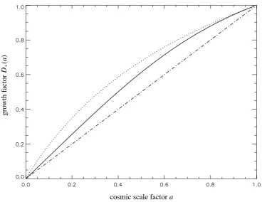
Figure 3.2.:The plot shows the growth functionD+(a) for three different cosmologies: A low-density model withΩm =0.3 and vanishing cosmological constantΩΛ=0.0 (dotted line), aΛCDM model (solid line) and
a SCDM model (dash-dotted line).
Once either the matter densityΩm has decreased sufficiently or the cosmological ΩΛhas started dominating the
Hubble expansion, as is the case for later times, the linear growth depends on the cosmic scale factoraaccording to:
δ(x,a)
δ(x,1) =a
g0(a)
g0(1) ≡D+(a), (3.38)
whereD+(a) is the solution to the growing mode of homogeneous structure formation. In general, the solution of equation (3.36) requires numerical integration. However, a good approximation tog0(a) for theΩ
m-dominated
phase of structure growth is provided byCarroll et al.(1992):
g0
(a)= 5 2Ωm(a)
"
Ω4/7
m (a)−ΩΛ(a)+ 1+
1 2Ωm(a)
!
1+ 1 70ΩΛ(a)
!#−1
. (3.39)
The growth functionD+(a) as a function of scale factoraof theΛCDM model, the SCDM model and a low density model without cosmological constantΛis depicted in Fig.3.2.
3.2.1.5. Velocities in the large-scale structure
In the previous section we focused on the evolution of the density contrast. However, for the analysis of large scale structure also the peculiar velocity field is of great importance. The linear velocity field can be easily calculated from equation (3.35) in Fourier space. For a harmonic perturbation with wave vectork, the peculiar velocityuis parallel tok:
u(k,t)=−ik
k2
dδ(k,t)
3.2.2 Zel’dovich approximation
As described above, in the linear regime the time evolution of the density fieldδis homogeneous and can therefore be expressed asδ(k,a)=D+(a)δ(k,1). With the definition of the Hubble function ˙a=aH(a) and the normalization of the growth function we hence yield:
u(k,a)=−iH(a)f(Ω)k
k2δ(k,a), (3.41)
where f describes the dependence of the equation of continuity on cosmic time and mainly depends on the mass densityΩm(Peebles 1980,Lahav et al. 1991):
f(Ω)= d lnδ d lna =
d lnD(a)
d lna 'Ωm(a)
0.6 (3.42)
The proper physical peculiar velocityδvis then obtained by multiplication with the cosmic scalefactora:
δv(k,a)=−ia H(a)f(Ω)k
k2δ(k,a). (3.43)
Investigation of peculiar velocity fields in our cosmic neighborhood is an interesting topic, since they can be used to test whether cosmic flows are irrotational and also to provide dynamical estimates ofΩmandσ8. For this reason,
reconstructions of the cosmic velocity field have been carried out e.g. with the POTENT algorithm proposed by
Bertschinger & Dekel(1989,1991).
3.2.2. Zel’dovich approximation
In the sections above, the fluid motions were described in an Eulerian coordinate system. However, it is possible to develop non-linear perturbation theory in the so-called Lagrangian framework. In this approach one follows the trajectories of individual particles or fluid elements rather than studying the dynamics of density and velocity fields (for a review of Lagrangian perturbation theory seeBuchert 1996,Bernardeau et al. 2002). To linear order this perturbation approach is equivalent to the Zel’dovich approximation, as proposed byZel’Dovich(1970). Here, the objects of interest are the particle trajectories, which link the initial particle positionsqto their positionsx(q,a) at a later time:
x(q,a)=q−D+(a)∇Ψ(q), (3.44) whereΨ(q) is the displacement potential given by the initial density contrast through a Poisson equation:
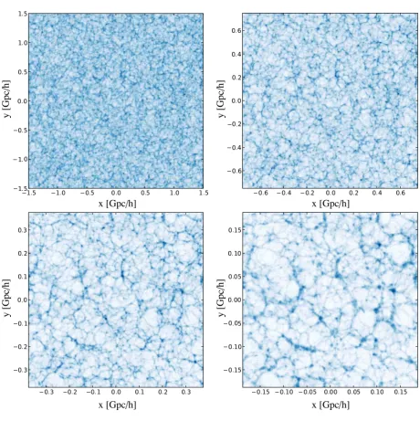
∇2Ψ(q)=δ(q). (3.45) Equation3.44, therefore, describes the particle dynamics as straight inertial motion in the direction of its initial velocity vector. Strictly speaking, extrapolation of peculiar velocities is only exact in one dimension. One di-mensional gravitational dynamics corresponds to following parallel sheets of matter, where the gravitational ac-celeration towards a sheet is independent of distance. Hence, the full equation of motion can be extrapolated from the particle’s initial peculiar velocity, as long as sheets do not cross (Peacock 1999). The dynamics de-scribed by equation (3.44) do not take into account gravitational interactions between individual particles. Thus, Zel’dovich’s approximation fails at sufficiently non-linear stages when particles are to be forming gravitationally bound objects instead of following straight lines. Nevertheless, Zel’dovich’s approximation provides interest-ing insight into the formation of the large scale cosmic web. Figure 3.3displays solutions of equation3.44for a set of 2563 particles. The initial density contrast δ(q) was generated from a multivariate normal distribution on a 2563 equidistant grid and according to a ΛCDM power-spectrum calculated according to the prescription presented in Eisenstein & Hu(1998) and Eisenstein & Hu(1999). Further, the set of cosmological parameters (Ωm=0.24,ΩΛ=0.76,Ωb=0.04,h=0.73, σ8 =0.74,ns=1) was adopted. The plots demonstrate the
filamen-tary cosmic web at four different resolutions.
To obtain the Eulerian density field at any epoch one exploits mass conservation [1+δ(q)]dq3=[1+δ(x)]dx3and uses the Jacobian of the transformation betweenqandx:
(1+δ(x))=(1+δ(q))dethδKi j−D+∂i∂jΨ
i−1
This result demonstrates that the tidal forces∂i∂jΨcause compressions of the cosmic density field (Schäfer 2009).
When using the three eigenvalues (λ1, λ2, λ3) of the Jacobian in equation (3.46) one can write:
(1+δ(x))= (1+δ(q))
(1−D+λ1)(1−D+λ2)(1−D+λ3)
. (3.47)
The details of structure growth in a particular region depends on the values (λ1, λ2, λ3) with (λ1 ≥λ2 ≥λ3). One
can see that ifλ1 >> λ2, λ3 then the gravitational collapse proceeds along one axis and forms a two dimensional
pancake. In regions whereλ1 ∼λ2 >> λ3the gravitational collapse is expected to be two dimensional and a one
dimensional filament will form. Forλ1 ∼ λ2 ∼ λ3 the gravitational collapse proceeds along all three axis and
will form a nearly spherical overdensity or halo. This behavior of gravitational structure formation lends itself to a cosmic web classification algorithm, which classifies different regions either as voids, sheets, filaments or halos. Such a dynamic web classification algorithm was proposed byHahn et al.(2007) and refined byForero-Romero et al.(2009). In chapter9an application of such a web classification method to observed data will be presented.
3.2.3. Numerical simulations of cosmic structure formation
The results presented above are only valid in the linear regime (|δ| 1). However, in the course of structure formation high density objects with overdensities|δ| 1 are formed, e.g. galaxies (δ'106), clusters of galaxies
(δ ' 100) and superclusters (δ '10). In these regimes, perturbation theory provides no valid description for the dynamics of these objects. In addition, non-linear structure formation generally proceeds heterogeneously, such, that the relationδ(x,a)=D+(a)δ(x) is violated. The non-linear dynamics yield strong coupling between different modesδ(k) in Fourier space, which does not permit a simple analytic approach. And thirdly, non-linear structure formation produces non-Gaussian features, due to phase correlations. This is due to the equation of continuity which prevents the density contrast to assume valuesδ <−1. The density fluctuation field therefore is bounded to small valuesδ >−1, but an upper bound does not exist. Thus, in the course of non-linear structure formation the distribution ofδnecessarily develops a non-vanishing skewness. For this reason, one cannot uniquely describe the statistical properties of the non-linear density field in terms of 2-point correlation functions or power spectraPδ(k).
In order to study the non-linear stages of cosmic structure formations, one usually relies on numerical simula-tion. These computer codes, the most notable of which is GADGET (Springel et al. 2001,Springel & Hernquist 2002), approximately solve the Vlasov equation (3.21), by following the trajectories of a set of discrete particles through phase space. In this fashion, one obtains a sampled representation of the phase space distributionf(r,p,t). Extensions to GADGET include baryonic dynamics, magnetic fields and cosmic rays. In this work some artificial galaxy catalogs based on simulations, carried out with GADGET, are used to test the presented large scale structure analysis methods.
3.3. Large scale structure
3.3.1. Distribution of matter in the Universe
3.3.1 Distribution of matter in the Universe