The modelling of corrective surface for gps height conversion in klang valley

(1)

33

THE MODELLING OF CORRECTIVE SURFACE FOR GPS

HEIGHT CONVERSION IN KLANG VALLEY

Abza Binti Khalid1 and Zainal Abidin Bin Md Som2

Faculty of Geoinformation and Real Estate, Universiti Teknologi Malaysia, Johor Malaysia Email: [email protected] and [email protected]

ABSTRACT

The modern technique in GPS-levelling plays a tremendous role of importance and alternative for practical height determination. One of the GPS-levelling contributions utilized is able to provide height information quickly. However, height given by GPS (h) has to be transformed to orthometric height (H) in order to use for the survey. In this case, the existence of the geoid undulation (N) is much needed and appreciated to allow the conversion processes occur. Although the theoretical relationships between these height types are simple in nature, practically are quite challenging due to numerous factors that cause discrepancies among the combined height data. This study focused on modelling the corrective surface in the form of geometric geoid for GPS height conversion in Klang Valley. Therefore, the relationship between h, H and N at 42 co-location points around Klang Valley was investigated in order to derive the corrective surface. Then, the method of least square adjustment (LSA) is used to determine the right parameter for corrective surface computation. Software will be developed to get the GPS conversion factor for Klang Valley. Analysis shows that the 4-parameter of simplified transformation model is the best parametric fit in Klang Valley area with Standard Deviation of 0.0215m and RMS of 0.0023m after fitting. Software named ‘KLANG VALLEY Corrective Surfacev1.0’ is developed by using Microsoft Visual Basic v6 to get the GPS conversion factor for Klang Valley.

Key Words: corrective surface, GPS-levelling, height determination, simplified transformation model

1.0

INTRODUCTION

For many decades ago, spirit-levelling was the only method used to provide height for control survey network and topographic elevation. The good thing about spirit-levelling is that it is highly precise and accurate. However, developments in Global Positioning System (GPS) have revolutionized the land surveying field, allowing the determination of horizontal position and also elevation or height. In this case, GPS technology provides an alternative and modernizing the method for height determination.

By comparing the GPS-levelling method with spirit-levelling, it shows that spirit-levelling is very accurate in obtaining a topographic height (in the form of orthometric height) but it is time consuming as well as labour-intensive. On the other hand, GPS-levelling provides several advantages as an alternative requires less labour, more flexible routine that did not subject to weather conditions so that the field work become a lot faster and easier to access. It is in line with the requirements of today's world that require efficiency and higher productivity, including the survey field.

However, the height values obtained from the GPS-levelling is different compared to the height of which is obtained from the spirit-levelling. Height of the GPS refers to the theoretical

(2)

surface of the earth known as the ellipsoid while height from spirit-levelling are normally requires an orthometric height. GPS height; h can be converted to orthometric height; H

exactly, if the separation distance between the geoid and ellipsoid (i.e. known as the geoid height; N) is known. Thus, surveyors need to have geoid information in order to convert the GPS height into orthometric height, so that the geoid has become an integral part of the geodetic infrastructure.

2.0

COMBINED ADJUSTMENT OF ELLIPSOIDAL, ORTHOMETRIC AND

GEOID

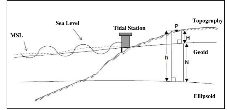
The combined use of GPS, levelling and geoid information has been used for various applications. Although these three types of height information are considerably different in terms of physical meaning, reference surface definition should fulfil the simple geometrical relationship:

h – H – N = 0 (eq. 2.1)

Where h is the geodetic height (ellipsoidal height) obtained from space-based system such as GPS, H is the normal height (orthometric height) usually obtained from spirit/precise levelling and N is the height anomaly obtained from a regional gravimetric geoid model or a global geopotential model depending on available data. The geometrical relationship between the triplets of height types illustrated to a point of P in Figure 2.1:

Figure 2.1: Relationships between the surface of topography, geoid and ellipsoid

2.1

Role of the Parametric Model

In practice, the implementation of the equation 2.1 is more complicated due to numerous factors that cause discrepancies when combining the heterogeneous heights. Fotopoulos G.

et al. (1999) described four main factors that cause discrepancies when combining the

heterogeneous heights. The statistical behaviour and modelling of the misclosure of equation 2.1 computed in a network of levelled GPS benchmarks, have been the subject of many studies which are often considerably different in terms of their research objectives.

In addition they also provided the references as representative to anybody who wants to study further on substitute the GPS height, h in equation 2.1 with altimetric observations and the orthometric height, H with Sea Surface Topography (SST). Meanwhile, Carina Raizner (2008) and Muhammad Firdaus Hashim (2010) add one more factors then Fotopoulos G. (2003, 2005) and Uliana Danila (2006) explain more about the factors which are:

MSL

Sea Level

Tidal Station

(3)

i. Random errors in the derived heights h, H, and N:

The covariance matrices for each of the height types (absolute or relative) are usually obtained from separate network adjustments of the individual height types. An overview of the main errors affecting the height data is provided in Fotopoulos (2003) and Uliana Danila (2006).

ii. Datum inconsistencies inherent among the height types:

Each of the triplets of height data refers to a different reference surface. For instance, GPS-derived heights refer to the geo-centre relative to which satellite orbits are determined. Orthometric heights, computed from levelling and gravity data, refer to a local vertical datum, which is usually defined by fixing one or more tide gauge stations.

Finally, the geoidal undulations interpolated from a gravimetrically derived geoid model refer to the reference surface used in the global geopotential model, which may not be the same as the one for the gravity anomalies.

iii. Systematic effects and distortions in the height data:

The systematic effects and distortions are primarily caused by long-wavelength geoid errors, which are usually attributed to the global geopotential model. Biases are also introduced into the gravimetric geoid model due to differences between data sources whose adopted reference systems are slightly difference.

In addition, systematic effects are also contained in the ellipsoidal heights, which are a result of poorly modelled GPS errors, such as atmospheric refraction (especially tropospheric errors). Although spirit-levelled height differences are usually quite precise, the derived orthometric heights for a region/nation are sometimes, the result of an over-constrained levelling network adjustment, which introduces distortions.

iv. Assumptions and theoretical approximations made in processing observed data:

Common approximations include neglecting SST effects or river discharge corrections for measured tide gauge values, which results in a deviation of readings from MSL. Other factors includes the use of approximations or inexact normal/orthometric height corrections and using normal gravity values instead of actual surface gravity values in computing orthometric heights. The computation of regional or continental geoid models also suffers from approximations in the gravity field modelling method used.

v. Instability of references station monuments overtime:

Temporal deviations of control station coordinates can be attributed to geodynamic effects such as post-glacial rebound, crustal motion and land subsidence. Most GPS processing software reduce all tidal effects when computing the final coordinate differences. To be consistent, the non-tidal geoid should be used.

2.2

Parametric Model Surface Fit

Most of the geoid evaluation studies were based on comparisons GPS-levelling data, have typically been designated to the incorporation of a parametric model in the combined adjustment of the heights based on equation:

(4)

Where h, H and N were as described previously, the parametric term a x describes the parameterized surface which are all possible datum inconsistencies and other systematic effects in datasets and v denotes the unmodelled residual random noise term.

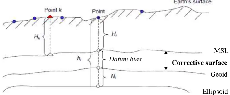
Figure 2.2: Illustrative view of GPS-levelling and the role of corrective surface

In this study, the vector of unknown parameters x for a selected parametric model are obtained via a common least square of ellipsoidal, orthometric and geoid height data over a network of collocated GPS-levelling bench-marks. Weighted observation which is another common method that has been employed extensively for computing the parametric model in least square co-location where the height differences are used.

According to Carina Raizner (2008) and Muhammad Firdaus Hashim (2010), in order to compensate for possible discrepancies, the incorporation of a parametric corrector surface model is essential in practice. The unknown model parameters can be estimated from a combined least square adjustment of ellipsoid, orthometric and geoid height data. There are various options to define a parametric surface model:

i. Polynomial Expansion of various order a. First-order polynomial

b. Second order polynomial c. Third-order polynomial d. Fourth-order polynomial

ii. Simplified / Similarity Transformation Model a. Classic four-parameter

b. Classic five-parameter c. Classic seven parameter

iii. Differential similarity

iv. Legendre polynomial

v. Fourier series

2.3

Modelling Options

In this study, mathematical model which are related to model the corrective surface are thoroughly studied. In practice of this study, the parametric models often used are:

MSL

Datum bias

]

“

“ellipsoid”

Ellipsoid

Geoid

(5)

i. Four-parameter model

a x= x1 + x2 cos φi cos i + x3 cos φi sin i + x4 sin φi (eq. 2.3)

ii. Five-parameter model extension

a x= x1 + x2 cos φi cos i + x3 cos φi sin i + x4 sin φi + x5 sin2 φi (eq. 2.4)

The equation (3) and (4) corresponds to the following datum transformation model for geoid undulation N, which is described as:

∆Ni = ∆a +∆Xo cos φi cosi + ∆Yo cos φi sin i + ∆Zo sin φi+ vi (eq. 2.5)

In addition, datum transformation model for equation (4) is denoted by a ∆fsin2 φI,

Where ∆Xo, ∆Yo, ∆Zo are the shift parameters between two parallel datum and ∆f, ∆a

are the changes in flattening and semi-major axis of corresponding ellipsoids.

iii. Seven-parameter model

a x = x1 cos φi cos i + x2 cos φi sin i + x3 sin φi + x4



+

x5



+ x6

+ x7

(eq. 2.6)

Where W = √ , e2 is the eccentricity, f is the flattening of the reference ellipsoid, and φ,  are the horizontal geodetic coordinates network.

The full form of design matrix would be given as follows:

2.3.1 Mathematical Model for Least Square Adjustment

Method of Linear Model is needed in order to obtain the value of x for that parameter described (Haji Abdul Wahid Idris & Halim Setan 2001):

i. The mathematical model for observation equation used in this programming is:

V = AX – Lb _{(eq. 2.7)}

Where V is a residual, A is a design matrix, X is a correction value and Lb is an observation data

P =Q-1 (eq. 2.8)

(6)

ii. The least-square adjustment (LSA) criteria is to obtain adjusted values of parameters that minimize sum of squares of weighted residuals (minimize VTPV)

VTPV = minimum

= (AX – L) T_{P (AX – L)} _{(eq. 2.9)}

= XT AT P A X – XTATPL - LTPAX + LTPL (eq. 2.10)

= XTATPAX – 2LTPAX + LTPL (eq. 2.11)

∂ (VT_{PV) / ∂X = 2A}T_{PAX – 2A}T_{PL =}₀ _{(eq. 2.12)}

Thus,

ATPAX – ATPL = 0 (eq. 2.13)

iii. The solution with the LSA concept was show in equal:

Normal equation : ATPAX=ATPL or NX = U (eq. 2.14)

Parameter : X=N-1Uif N = ATPA and U = ATPLb (eq. 2.15)

Thus, X = (ATPA)-1 ATPL (eq. 2.16)

Residual : V=AX-Lb (eq. 2.17)

Adjusted Observation: La = Lb + V (eq. 2.18)

Then, equation 2.2 followed by equation 2.3, 2.4, 2.6 were calculate in Fortran Programming Language. Then equation 2.19 used to model the geometric geoid.

2.4

Corrective Surface by Geoid Fitting

Datum bias is the difference between the gravimetric geoid and local MSL (See Figure 2.2). Hence fitting the gravimetric geoid onto the local MSL which is National Geodetic Vertical Datum (NGVD) will minimize the effect of datum biases. Usually, this is done by fitting the surface based on reference points which is the gravimetric geoid fitted to the geometric model by using the equation 2.2.

The fitting of gravimetric geoid to GPS geoid surface, typically available in grid form and involve modelling the differences. By adding the correction (ε) to the original gravimetric geoid will fit the gravimetric model to the NGVD. The equation (2.19) indicates about corrective surface:

NGPS = h-H- ε (eq. 2.19)

3.0

Practical Application of GPS/levelling Network (MyGEOID)

In Malaysia starting in 2002, JUPEM has undertaken the project of mapping the geoid with the main objective to produce high precision geoid model in order to determine the geoid height in the whole country with the aim to make the best possible national geoid model, see Ahmad Fauzi Nordin et al. (2005).

The mathematical model used in determination of MyGEOID is based on a combination of spherical harmonic potential coefficient and terrestrial gravity data. The formula used to compute the gravimetric geoid heights, see Ahmad Fauzi Nordin et al. (2005); Md. Nor Kamarudin & Ernest Khoo Hock Don (1999).

(7)

The EMGEOID05 geoid model for Sabah and Sarawak is fitted to the Sabah Datum 1997 which is based on 10 years observation (1988-1997) at Kota Kinabalu Tide Gauge Station. The WMGEOID04 geoid model is fitted to the National Geodetic Vertical Datum (NGVD) in Peninsular Malaysia, which is based on 10 years observation (1984-1993) of the MSL at Port Klang (See KPUP 2005 for more details).

Figure 3.1: WMGEOID04 for Peninsular Malaysia with contour interval every 1m. The circle indicates the areas involved for the case study

4.0

DISCUSSION

Figure 4.1: Figure 4 shows the distribution of 42 co-location point in Klang Valley

(8)

4.1

The Statistics Before Fitting

Table 4.1 below shows the statistics of 42 co-location point and the datum inconsistencies before fitting which were calculated in Microsoft Office Excel.

Table 4.1: The statistics of data 42 co-location points and datum inconsistencies

42 co-location points

Ellipsoidal Height (h)

Orthometric

Height (H) WMGEOID04 (N)

Datum Inconsistencies

(h-H-N)

Minimum -0.870 2.261 -4.959 1.2230

Maximum 70.294 72.266 -2.884 1.3260

Mean 23.898 26.519 -3.899 1.2781

SD 23.121 22.845 0.502 0.0245

RMS 27.691 29.267 3.954 1.2772

4.2

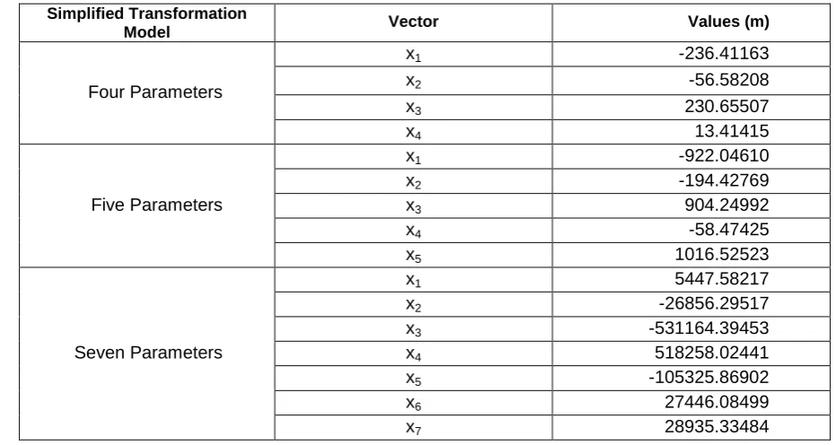
The Vector of Estimated Transformation Parameters

The values of vector for each estimated transformation parameter model of four, five and seven parameters were determined by LSA processes using Fortran Programming. The values are presented in Table 4.2.

Table 4.2: Values of the vector for each estimated transformation parameters

Simplified Transformation

Model Vector Values (m)

Four Parameters

x1 -236.41163

x2 -56.58208

x3 230.65507

x4 13.41415

Five Parameters

x1 -922.04610

x2 -194.42769

x3 904.24992

x4 -58.47425

x5 1016.52523

Seven Parameters

x1 5447.58217

x2 -26856.29517

x3 -531164.39453

x4 518258.02441

x5 -105325.86902

x6 27446.08499

x7 28935.33484

4.3

Accesing the Simplified Transformation Model Performance

Each vector of estimated transformation parameters were then used in equation 2.3, 2.4 and 2.6 respectively. This was also then calculated in Fortran Programming Software. The results were then used to model the Geometric Geoid of each parameter model by using Microsoft Office Excel 2007.

(9)

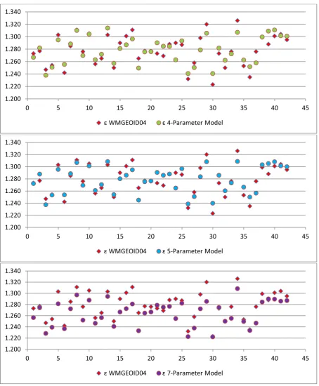
Figure 4.2: Comparison using analysis of empirical statistics between εWMGEOID04 with each of parametric model of four, five and seven.

Referring to Figure 4.2, the optimum values from four and five parameter are represented by and symbol respectively. These are closer to the actual values (i.e. height misclosures of WMGEOID04 represented by symbol) compared to values shown by seven parameters represented by symbol. Thus, to gain the more accurate or precise value, numerical statistical test need to do and the result as shown on the Table 4.3.

Table 4.3 summarize that Root Mean Square (RMS) of four and five parameter values is same (1.2748m). Their result is very close to gravimetric model (1.2772m) compared to 7

1.200 1.220 1.240 1.260 1.280 1.300 1.320 1.340

0 5 10 15 20 25 30 35 40 45

ε WMGEOID04 ε 4-Parameter Model

1.200 1.220 1.240 1.260 1.280 1.300 1.320 1.340

0 5 10 15 20 25 30 35 40 45

ε WMGEOID04 ε 5-Parameter Model

1.200 1.220 1.240 1.260 1.280 1.300 1.320 1.340

0 5 10 15 20 25 30 35 40 45

(10)

parameter RMS values (1.2617m). In this case we should refer to the values of standard deviation (SD).

Table 4.3: Statistical results of 42 co-location points used in adjustment before & after fitting

42 co-location

points

ε

WMGEOID04

Simplified Transformation Model

ε

4-Parameters

ε

5-Parameters

ε

7-Parameters

Minimum 1.2230 1.2381 1.2373 1.2221

Maximum 1.3260 1.3139 1.3087 1.3083

Mean 1.2781 1.2781 1.2781 1.2645

SD 0.0245 0.0215 0.0217 0.0220

RMS 1.2772 1.2748 1.2748 1.2617

RMS Difference Compared to The

Absolute Value 0.0024 0.0024 0.0155

According to the SD, it shows that the values of four parameter model contain the minimum value of 0.0215m compared to other values which are 0.0217m and 0.0220m for five and seven parameter respectively. This proves that the 4 parameters model are the best model fitted in this study.

4.3.1 Interpolation method

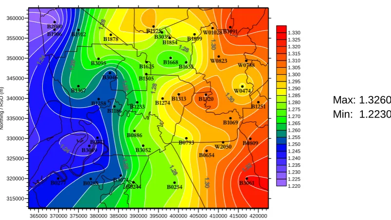
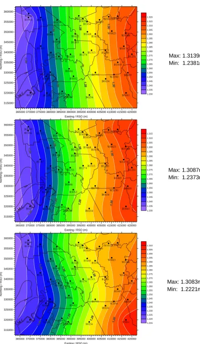
Contour modelling of height misclosures for εWMGEOID04 and every simplified transformation model can be referred to Figure 4.3 and 4.4. In summary, contour height is at interval of every 5 mm which is 0.005m. Value differences for every contour line are represented by colour scale (at right hand side).

The kriging interpolation technique was used to create a continuous surface to be used in Golden Surfer v 8. Kriging is a geostatistical approach to interpolate data based upon spatial variance. It is proven useful and popular in many fields in geodesy as well. This method has become an extremely important interpolation tools in GIS. As such, it had receives lot of attention from scientists and software producers as defined in Uliana Danila (2006).

Figure 4.3: Height misclosures for WMGEOID04. Contour interval every 5mm (0.005m) refer to the calculation of ∆N = hi-Hi-NWMGEOID04

365000 370000 375000 380000 385000 390000 395000 400000 405000 410000 415000 420000

Easting / RSO (m)

315000 320000 325000 330000 335000 340000 345000 350000 355000 360000 N o rt h in g / R S O ( m ) B0244 B0254 B0277 B0285 B0654

B0771 B0793 B0809

B0886

B1069

B1186 B1233 B1251

B1258 B1274B1313 B1320 B1367

B1505

B1625 B1668B1635 B1854

B1878 B1899

B1906 B1912 B1975 B1991

(11)

Figure 4.4: Height misclosures for each simplified transformation model of four, five and seven model respectively. Contour interval every 5mm (0.005m)

365000 370000 375000 380000 385000 390000 395000 400000 405000 410000 415000 420000 Easting / RSO (m)

315000 320000 325000 330000 335000 340000 345000 350000 355000 360000 N o rt h in g / R S O ( m ) B0244 B0254 B0277 B0285 B0654

B0771 B0793 B0809

B0886

B1069

B1186 B1233 B1251

B1258 B1274B1313 B1320 B1367

B1505

B1625 B1668B1635 B1854

B1878 B1899

B1906 B1912 B1975 B1991

B2000 B3039 B3046 B3052 B3061 B3074 B3089 B3095 W01028 W0474 W0788 W0823 W2050 1.230 1.235 1.240 1.245 1.250 1.255 1.260 1.265 1.270 1.275 1.280 1.285 1.290 1.295 1.300 1.305 1.310 1.315 1.320

365000 370000 375000 380000 385000 390000 395000 400000 405000 410000 415000 420000

Easting / RSO (m)

B0771 B0793 B0809

B0886

B1069

B1186 B1233 B1251

B1258 B1274B1313 B1320 B1367

B1505

B1625 B1668B1635 B1854

B1878 B1899

B1906 B1912 B1975 B1991

B2000 B3039 B3046 B3052 B3061 B3074 B3089 B3095 W01028 W0474 W0788 W0823 W2050 1.230 1.235 1.240 1.245 1.250 1.255 1.260 1.265 1.270 1.275 1.280 1.285 1.290 1.295 1.300 1.305 1.310 1.315

365000 370000 375000 380000 385000 390000 395000 400000 405000 410000 415000 420000

Easting / RSO (m)

B0771 B0793 B0809

B0886

B1069

B1186 B1233 B1251

B1258 B1274B1313 B1320 B1367

B1505

B1625 B1668B1635 B1854

B1878 B1899

B1906 B1912 B1975 B1991

B2000 B3039 B3046 B3052 B3061 B3074 B3089 B3095 W01028 W0474 W0788 W0823 W2050 1.215 1.220 1.225 1.230 1.235 1.240 1.245 1.250 1.255 1.260 1.265 1.270 1.275 1.280 1.285 1.290 1.295 1.300 1.305 1.310 Max: 1.3139m Min: 1.2381m

Max: 1.3087m Min: 1.2373m

(12)

4.4

Fitting of the Corrective Surface

Next, the values of each height misclosures summarized on Table 4.3 used to determine the

N value for each parameter (i.e. Geometric Geoid) by using the equation 2.19. This was calculated using Microsoft Excel. The summary of result is shown in Table 4.4.

Table 4.4: Statistical results of Geometric Geoid

42 co-location

points NWMGEOID04

Geometric Geoid

N4 N5 N7

Minimum -4.9590 -4.9768 -4.9758 -4.9581

Maximum -2.8840 -2.8650 -2.8667 -2.8663

Mean -3.8990 -3.8991 -3.8991 -3.8855

SD 0.5022 0.5022 0.5022 0.5021

RMS 3.9538 3.9515 3.9516 3.9383

RMS Difference Compared to The

Absolute Value 0.0023 0.0024 0.0155

Based on results tabulated in Table 4.4, it shows that standard deviation (SD) of seven parameter model has value differences of -0.0001 compared to four and five parameter values which contain the same number with absolute value of 0.5022m respectively.

While refer to the RMS value of each parameter (compared with RMS of absolute value), it shows that the Geometric Geoid of four parameter contain the lowest value than five parameter with only slight difference of +0.0001m and 0.0155m for seven parameter model. As such, the results prove again that the 4 parameter models are the best model fitted in this study.

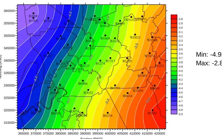
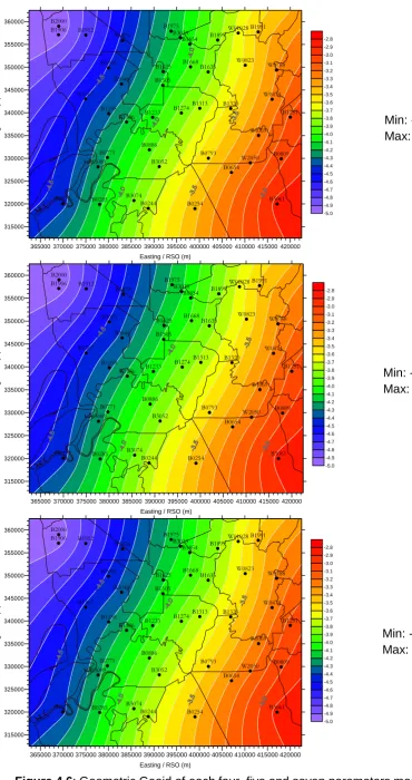
After that, modelling for every geometric geoid is shown by Figure 4.5 and 4.6. In summary, contour interval is at every 10cm (0.100m). The differences of value in every contour line are given in colour scale (right hand side).

Figure 4.5: Gravimetric Geoid for WMGEOID04 which is the actual geoid in Klang Valley. Contour interval every 10cm (0.100m)

365000 370000 375000 380000 385000 390000 395000 400000 405000 410000 415000 420000 Easting (RSO) 315000 320000 325000 330000 335000 340000 345000 350000 355000 360000 N o rt h in g ( R S O ) B0244 B0254 B0277 B0285 B0654

B0771 B0793 B0809

B0886

B1069

B1186 B1233 B1251

B1258 B1274B1313 B1320 B1367

B1505

B1625 B1668B1635 B1854

B1878 B1899

B1906 B1912 B1975 B1991

(13)

365000 370000 375000 380000 385000 390000 395000 400000 405000 410000 415000 420000 Easting / RSO (m)

B0771 B0793 B0809

B0886

B1069

B1186 B1233 B1251

B1258 B1274B1313 B1320 B1367

B1505

B1625 B1668B1635 B1854

B1878 B1899

B1906 B1912 B1975 B1991

B2000 B3039 B3046 B3052 B3061 B3074 B3089 B3095 W01028 W0474 W0788 W0823 W2050 -5.0 -4.9 -4.8 -4.7 -4.6 -4.5 -4.4 -4.3 -4.2 -4.1 -4.0 -3.9 -3.8 -3.7 -3.6 -3.5 -3.4 -3.3 -3.2 -3.1 -3.0 -2.9 -2.8

365000 370000 375000 380000 385000 390000 395000 400000 405000 410000 415000 420000 Easting / RSO (m)

B0771 B0793 B0809

B0886

B1069

B1186 B1233 B1251

B1258 B1274B1313 B1320 B1367

B1505

B1625 B1668B1635 B1854

B1878 B1899

B1906 B1912 B1975 B1991

B2000 B3039 B3046 B3052 B3061 B3074 B3089 B3095 W01028 W0474 W0788 W0823 W2050 -5.0 -4.9 -4.8 -4.7 -4.6 -4.5 -4.4 -4.3 -4.2 -4.1 -4.0 -3.9 -3.8 -3.7 -3.6 -3.5 -3.4 -3.3 -3.2 -3.1 -3.0 -2.9 -2.8

365000 370000 375000 380000 385000 390000 395000 400000 405000 410000 415000 420000 Easting / RSO (m)

B0771 B0793 B0809

B0886

B1069

B1186 B1233 B1251

B1258 B1274B1313 B1320 B1367

B1505

B1625 B1668B1635 B1854

B1878 B1899

B1906 B1912 B1975 B1991

B2000 B3039 B3046 B3052 B3061 B3074 B3089 B3095 W01028 W0474 W0788 W0823 W2050 -5.0 -4.9 -4.8 -4.7 -4.6 -4.5 -4.4 -4.3 -4.2 -4.1 -4.0 -3.9 -3.8 -3.7 -3.6 -3.5 -3.4 -3.3 -3.2 -3.1 -3.0 -2.9 -2.8 Min: -4.9768m Max: -2.8650m Min: -4.9758m Max: -2.8667m Min: -4.9581m Max: -2.8663m

(14)

Surface for each parametric model plotted as below:

-4.9 -4.8 -4.7 -4.6 -4.5 -4.4 -4.3 -4.2 -4.1 -4.0 -3.9 -3.8 -3.7 -3.6 -3.5 -3.4 -3.3 -3.2 -3.1 -3.0 -2.9

(15)

Figure 4.7: Surface Plotted for each adjusted geometric geoid (N4, N5 and N7) in perspective view respectively. The range of N is between -5 and -2m

4.5

Writing a Program

Understanding on FORTRAN and Visual Basic programming language is very important to be familiar with its function. Step by step in writing a program can be defined as Figure 4.8:

Figure 4.8: Flowcharts on steps to write a Program

STEP

1

• Describes the problems

STEP

2

•Analysis the programs

STEP

3

•Design a general of logic programs

STEP

4

•Design a detailed of logic programs

STEP

5

•Code the programs

STEP

6

•Test and debug the programs

STEP

7

(16)

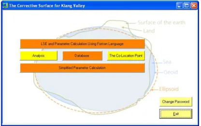
Figure 4.9: Main Menu from Software Development of ‘KLANG VALLEY Corrective Surface

v1.0’

5.0

CONCLUSION

The new geometric geoid model has been computed covering Klang Valley by using the data from WMGEOID04, height modernization on precise levelling network and GPS-levelling which consists of the 42 co-location points. The datum inconsistencies which lie between the geoid and MSL have been removed via the simplified transformation of four, five and seven parameter and residual have been eliminated from the original GPS/levelling data.

Therefore, the use of combined GPS/precise levelling/geoid networks provides a very attractive evaluation scheme for the accuracy of gravimetric and geometric geoid models. Besides, the use of parametric correction model can absorb the errors from random errors in the derived heights (h, H and N), datum inconsistencies inherent among the height types, systematic effects and distortions in the height data, assumptions and theoretical approximations made in processing observed data.

The geometric geoid produced covers the area in RSO Coordinate between 312,500 North and 362,500 North; and 362,500 East and 422,500 East of grid size 1.2cm x 1.2cm (5km x 5km). The range of height values for four-parameter geometric geoid is between -2.8650m meters to -4.9768m meters. However, this absolute verification does not show the real potential of the geoid models, so the final residuals are not the exact error of the gravimetric geoid model. The negative sign in the height of the geometric geoid means that the surface of the geoid is below the ellipsoid surface.

In addition, software of ‘KLANG VALLEY Corrective Surface v1.0’ of geometric geoid is specially developed for Klang Valley area because the data that being used are from a series data of 42 co-location points related in Klang Valley. Therefore, the data of GPS levelling or the Geographical coordinate which areas outside the Klang Valley are not suitable to use this program.

5.1

Recommendation and Further Research

In addition, further research can be done to gain the data of GPS height is being practice by Licensed Land Surveyor (LS) or any companies involved in GPS-levelling around Kuala Lumpur and Selangor to compare the result that have been processed in actual height data from their previous projects with data that produced from the developing software. Hopefully it will help to improve program of corrective surface.

As mentioned in Section 2.2, the modelling options are various and the results of the combined height adjustment are directly related to the choice of the parametric surface model. The suggestion here is to make the comparison between the best four parameter of simplified transformation model in this study with other parametric surface model like a group of Polynomial Expansion of first, second, third and fourth order polynomial or others group parametric model like Differential Similarity, Legendre Polynomial or Fourier series.

(17)

ACKNOWLEDGEMENTS

The authors acknowledge that the Department of Survey and Mapping Malaysia (JUPEM) are the data sources of 42 co-location point in Klang Valley

REFERENCES

Ahmad Fauzi Nordin, Samad Hj. Abu, Chang Leng Hua and Soeb Nordin (2005). Coordinates – Positioning, Navigation and Beyond. Malaysia Precise Geoid (MyGEOID). Vol 1 Issue 4, September 2005: 30 - 37

Carina Raizner (2008). A Regional Analysis of GNSS-levelling. Universiti of Stuttgart, German. Diploma Thesis.

Haji Abdul Wahid Idris and Halim Setan (2001). Pelarasan Ukur. Dewan Bahasa dan Pustaka. Kuala Lumpur

Fotopoulos G., Kotsakis C. and Sideris M.G. (1999). Evaluation of Geoid Models and Their Use in Combined GPS/Levelling/Geoid Height Network Adjustments. Technical Reports Department of Geodesy and Geoinformatics, Universiti of Calgary, Canada. Report No. 1999.4

Fotopoulos G., Kotsakis C. and Sideris M.G. (2005). Estimation of Variance Components Through a Combined Adjustment of GPS, Geoid and Levelling Data. International Association of Geodesy Symposia, Vol. 128, Symposium G04 : 440-445

Fotopoulos G. (2003). An Analysis on the Optimal Combination of Geoid, Orthometric and Ellipsoidal Height Data. PhD. Thesis, University of Calgary, Department of Geomatics Engineering, Report No. 20185

Fotopoulos G. (2005). Calibration of Geoid Error Models via a Combined Adjustment of Ellipsoidal, Orthometric and Gravimetric Geoid Height Data. Journal of Geodesy, Springer-Verlag, Vol. 79 Numbers 1-3 : 111-123,

Md. Nor Kamarudin and Ernest Khoo Hock Don (1999). Perkembangan Dalam Penentuan Model Geoid Masa Kini. Buletin Geoinformasi: Jld. 3, No.1, Sept. Penerbitan Akademik Fakulti Kejuruteraan & Sains Geoinformasi, Universiti Teknologi Malaysia: 22-36

Muhammad Firdaus Hashim (2010). The Estimation of Height Conversion Parameters for

Global Positioning System (GPS) Height Transformation. Universiti Teknologi Malaysia.

B.Sc. Thesis: Fakulti Kejuruteraan dan Sains Geoinformasi.

Pekeliling Ketua Pengarah Ukur dan Pemetaan Malaysia Bil. 10, Tahun 2005 (KPUP 2005).

Garis Panduan Penggunaan Model Geoid Malaysia (MyGEOID). Rujukan JUPEM 18/7/2.148

(87), 6 September 2005.

(18)

AUTHORS

Abza Binti Khalid is a final year undergraduate student who undertaking Bachelor in Engineering (Geomatic) at Faculty of Geoinformation and Real Estate, Universiti Teknologi Malaysia. Her research interest is geodesy and mathematics.