A new fourth-order embedded method based on the harmonic mean

A New Fourth-Order Embedded Method

Based on the Harmonic Mean

Nazeeruddin Yaacob & Bahrom Sanugi

Department of Mathematics

Universiti Teknologi Malaysia

81310 UTM Skudai, Johor, Malaysia

Abstract In this paper we formulate an embedded method based on harmonic and arithmetic means of order 4. This method together with RK-Harmonic scheme may be used to estimate the solutions of initial value problems. The absolute stability region of this scheme is also studied and we conclude with a numerical example to justify the effectiveness of the method.

Keywords Harmonic Mean, Runge-Kutta method, stability, error control.

Abstrak Dalam kertas ini kami rumuskan satu kaedah terbenam berperingkat 4 yang berasaskan min harmonik dan min aritmetik. Kaedah ini berserta de-ngan skema RK-Harmonik boleh digunakan bagi mede-nganggarkan penyelesaian kepada masalah nilai awal. Rantau kestabilan untuk skema ini juga dikaji dan kita simpulkan dapatan ini dengan satu contoh masalah sebagai mengesahkan keberkesanan kaedah ini.

Katakunci Min-Harmonik, Kaedah Runge-Kutta, kestabilan, kawalan ralat.

1

Introduction

One of the difficulties in implementing the classical Runge-Kutta method is the absence of estimation of errors procedure in computating the numerical solutions. Several methods have been developed to overcome these weaknesses, specifically this is done by introducing the procedure that can estimate the errors in the results. Amongst them are methods developed by Merson, Scraton [2] and Fehlberg [1]. Related work was carried out by Sanugi [3], who introduced a fourth order AGM method which is based on geometric mean plus a fourth order method based on arithmetic mean. Both methods used the common k’s,

ki, i = 1,2,3,4 . Similarly, we develop a much simpler embedded method of fourth order

2

Formulation of Fourth Order RK-HM-AM Scheme

Sanugi and Evans [4] had introduced a fourth order RK formula based on the harmonic mean with parameters

a1= 1/2, a2=−1/8, a3= 5/8, a4=−1/4, a5= 7/20,anda6= 9/10,

where

k1=f(xn, yn), (1)

k2=f(xn+a1h, yn+a1hk1), (2)

k3=f(xn+ (a2+a3)h, y)n+a2hk1+a3hk2), (3)

k4=f(xn+ (a4+a5+a6)h, yn+a4hk1+a5hk2+a6hk3), (4)

and

y_nHM₊₁ =yn+

2h

3

k1k2

k1+k2

+ k2k3

k2+k3

+ k3k4

k3+k4

. (5)

Using the common aiwe try to formulate another scheme which combines both arithmetic

mean (AM) and harmonic mean (HM). We propose the following scheme:

y_nAHM₊₁ =yn+h

h

d1k1+d2k2+d3k3+d4k4+d5

k1k2

k1+k2

+d6

_k

2k3

k2+k3

+d7

_k

3k4

k3+k4

i

, (6)

with constants dj,j= 1,2, . . . ,7, that are still undetermined andki+ki+16= 0.

By consideringy0_{=f(y), wheref is a function ofy only andy is either monotonically}

increasing or decreasing, we expand the equations (6) andy(xn+h) using the Taylor series

expansion. Using a symbolic computational package, MATHEMATICA, we compare the coefficients forh,h2,h3, andh4 to obtain the following seven linear equations:

hf : 1−d1−d2−d3−d4−

d5

2 −

d6

2 −

d7

2 = 0 (7)

h2fy:

1 2−

d2

2 −

d3

2 −d4−

d5

8 −

d6

8 −

d7

8 = 0 (8)

h3f fy2:

1 6−

5d3

16 − 5d4

8 +

d5

32− 5d6

64 − 13d7

64 = 0 (9)

h3f2fyy:

1 6− d2 8 − d3 8 − d4 2 − d5 32− d6 16− 5d7

32 = 0 (10)

h4f f_y3: 1 24−

9d4

32 −

d5

128− 7d7

128 = 0 (11)

h4f2fyfyy:

1 6−

15d3

64 − 25d4

32 +

d5

64− 15d6

256 − 53d7

256 = 0 (12)

Solving (7)-(13) yields

d1= 0, d2=

1 6, d3=

1

6, d4= 0, d5= 2

3, d6= 0, d7= 2 3. Thus, equation (6) becomes

yAHM_n+1 =yn+h

h₁

6k2+ 1 6k3+

2 3

_k

1k2

k1+k2

+2 3

_k

3k4

k3+k4

i

. (14)

We shall refer this formula as RK-HM-AM in the following sections.

3

Stability Analysis for RK-HM-AM Scheme

We used the test equation y0 _{= λy, λ is a constant, to obtain absolute stability regions}

for both RK-HM and RK-HM-AM methods. Substituting λ0

n = λyn in ki, i = 1,2,3,4

respectively, we obtain

k1=f(yn) =λyn (15)

k2=f

yn+

hk1

2

=λyn

1 +λh 2

(16)

k3=f

yn−

hk1

8 + 5hk2

8

=λyn

1 +λh 2 +

5(λh)2

16

(17)

k4=f

yn−

hk1

4 + 7hk2

20 + 9hk3

10

=λyn

1 +λh+5(λh)

2

8 + 9(λh)3

32

(18)

Substituting these values in (5) and (14) will yield

yHM n+1

yn

= 1 +λh+(λh)

2

2 + (λh)3

6 + (λh)4

24 − 3(λh)5

128 +O(h

6_{) (19)}

and

yAHM n+1

yn

= 1 +λh+(λh)

2

2 + (λh)3

6 + (λh)4

24 −

47(λh)5 3072 +O(h

6_{). (20)}

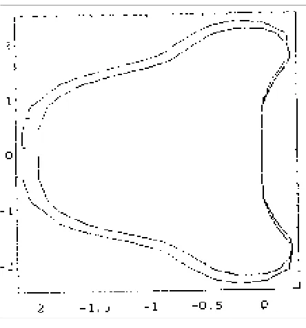
If λh = z, then (19) and (20) are the stability polynomials of RK-HM and RH-HM-AM respectively,

QHM(z) =y

HM n+1

yn

= 1 +z+z

2 2 + z3 6 + z4 24− 3z5

128+O(h

6_{) (21)}

and

QAHM(z) =y

AHM n+1

yn

= 1 +z+z

2 2 + z3 6 + z4 24− 47z5

3072+O(h

6_{) (22)}

Figure 1: Absolute stability regions for the RK-HM (smaller) and RK-HM-AM methods

4

Error Estimation

In RK-Fehlberg scheme [1], estimated errors are obtained by taking the difference of fifth order RK and fourth order RK solutions. While in Merson scheme [2], estimated errors are obtained by taking difference of solutions of two fourth order methods with different number of stages. In our scheme, we used two methods (5) and (14) sharing the samea’s and k’s (equal number of stages) but having different form ofyn+1.

Local truncation errors (LTE) for RK-HM method is given as,

LTE(HM) =y(xn+h)−ynHM+1 =

₆₁

1920f f

4

y −

61 7680f

2_f2

yfyy−

17 960f

3_f2

yy

− 1

640f

3

fyfyyy−

1 2880f

4

fyyyy

h5+O(h6) (23)

while LTE for RK-HM-AM is given as

LTE(AHM) =y(xn+h)−yAHMn+1 =

₁₂₁

5120f f

4

y−

61 7680f

2_f2

yfyy−

17 960f

3_f2

yy

− 1

640f

3_f

yfyyy−

1 2880f

4_f

yyyy

h5+O(h6) (24)

Now, subtracting (23) from (24) yields,

or

f fy4h5=

3072 25 y

HM

n+1 −yAHMn+1

. (25)

Iffyy= 0, thenfyyy=fyyyy= 0, i.e. f is a linear function iny. Thus using (25) we obtain

LTE(HM) = 3.904 ynHM+1−ynAHM+1

(26)

and

LTE(AHM) = 2.904 y_nHM₊₁ −y_nAHM₊₁ (27) This implies that the estimated errors of RK-HM and RK-HM-AM are approximately four and three times the difference of both methods.

5

Numerical Results

The folowing example shows how error estimation and error control are used.

y0= 1

y, y(0) = 1, 0≤x≤1.25.

The exact solution isy(x) =√2x+ 1.

Using error estimation = 2.904 yHM_−yAHM_{, with error tolerance = 10}−6 _{we obtain}

the following results.

COMPUTER OUTPUT

ERROR TOLERANCE =.1D-05 X0 = 0.00000

Y0 = 0.1000000D+01

Table 1: H = 0.1250000

X EXACT SOLN YAHM |ERROR| |EST. ERROR|

0.1250 1.1180340 1.1180337 0.3344949E-06 0.5463125E-06 0.2500 1.2247449 1.2247443 0.6111894E-06 0.2171449E-06 0.3750 1.3228757 1.3228750 0.6969985E-06 0.1036227E-06 0.5000 1.4142136 1.4142128 0.7167391E-06 0.5678877E-07 0.6250 1.5000000 1.4999993 0.7110623E-06 0.3479989E-07

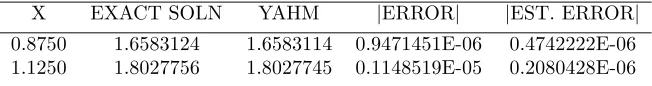
Table 2: H= 0.2500000

X EXACT SOLN YAHM |ERROR| |EST. ERROR|

6

Conclusion

In this paper we have developed an embedded method of order 4 based on arithmetic and harmonic means. By having equal number of stages and different form ofyn+1, we are able

to reduce the cost of computation for complicated function. From Table 1, obviously, for the first few steps, the absolute errors are approximately closed to the estimated errors. Con-sequently, the former become larger due to the effect of global errors. These are expected. Further research is recommended especially for problem of the type

y0=f(x, y), y(a) =η, a≤x≤b.

References

[1] R.L. Burden and J.D. Faires,Numerical Analysis, PWS Publishing Co., 1993.

[2] J.D. Lambert,Computational Methods in Ordinary Differential Equations, John Wi-ley & Sons, Great Britain, 1973.

[3] B.B. Sanugi, Ph.D. Thesis Loughborough University of Technology, 1986.