University of Huddersfield Repository
Newton, Andrew D., Hirschfield, Alex, Armitage, Rachel, Rogerson, Michelle, Monchuk, Leanne
and Wilcox, Aidan
Evaluation of Licensing Act: Measuring Crime and Disorder in and around Licensed Premises,
Research Study SRG/05/007 Technical Annex prepared for the Home Office
Original Citation
Newton, Andrew D., Hirschfield, Alex, Armitage, Rachel, Rogerson, Michelle, Monchuk, Leanne
and Wilcox, Aidan (2008) Evaluation of Licensing Act: Measuring Crime and Disorder in and
around Licensed Premises, Research Study SRG/05/007 Technical Annex prepared for the Home
Office. Research Report. University of Huddersfield.
This version is available at http://eprints.hud.ac.uk/id/eprint/9553/
The University Repository is a digital collection of the research output of the
University, available on Open Access. Copyright and Moral Rights for the items
on this site are retained by the individual author and/or other copyright owners.
Users may access full items free of charge; copies of full text items generally
can be reproduced, displayed or performed and given to third parties in any
format or medium for personal research or study, educational or notforprofit
purposes without prior permission or charge, provided:
•
The authors, title and full bibliographic details is credited in any copy;
•
A hyperlink and/or URL is included for the original metadata page; and
•
The content is not changed in any way.
For more information, including our policy and submission procedure, please
contact the Repository Team at: [email protected].
Evaluation of Licensing Act:
Measuring Crime and Disorder in and around
Licensed Premises
Research Study SRG/05/007
Final Report Prepared for the Home Office
Technical Annex
Dr Andrew Newton, Professor Alex Hirschfield, Dr. Rachel
Armitage, Michelle Rogerson, Leanne Monchuk and Dr
Aidan Wilcox
March 2008
The views expressed in this report are those of the authors, not necessarily those of the
Home Office (nor do they reflect Government policy).
This report was submitted July 2007.
Executive Statement
The Licensing Act 2003 (hereafter referred to as the Act), which came into effect on 24th November 2005, represented a major change to the sale of alcohol in England and Wales, by potentially allowing licensed premises to sell alcohol for up to 24 hours, 7 days per week.
The introduction of the Act brought with it a range of additional measures. These included an expansion of police powers to close areas or particular premises, specific offences relating to the sale of alcohol to children and a new mechanism for reviewing the granting of licenses that takes into account crime prevention, public safety public nuisance and child protection.
Table of contents
List of tables
List of appendices
1. Introduction
Research aims Research design
Randomised control trials (RCT) Matched pairs
Longitudinal status comparisons History
Regression to the mean Research context
Scale of analysis Timescale
Research approach
A note on the licensed premises data
2. Crime data analysis
Description of the data Data accuracy and reliability
Data capture and cleaning Data coding
Validation of location data Methodology
Distribution of offences (daily, weekly, monthly and by time of day) Crime rates
Percentage change Proportional change Victim profile
‘Alcohol’ and ‘domestic violence’ flags GIS analysis
Hot spot analysis Crime ratios
Resource Targeting Tables
Additional hours used (sample premises visited) Additional hours applied for (estimated for all premises) Limitations and analysis not considered
3. Disorder data analysis
Data accuracy and reliability Data capture and cleaning Data coding
Validation of location data Methodologies
Distribution of offences (daily, weekly, monthly and by time of day) Incident rates
Percentage change Proportional change GIS analysis Incident ratios
Limitations and analysis not considered
4. Health data analysis
Description of the data Data accuracy and reliability
Data capture and cleaning Data coding
Data completeness Methodologies
Distribution of incidents by month and year Percentage change
Distribution of incidents by time of day Victim profile
Limitations and analysis not considered
5. Supplementary analysis
Statistical significance tests
Serious and other violence against the person Weekday and weekend comparisons
Synthesis maps
6. Qualitative analysis
Timescale
Participant observation Semi-structured interviews
Phase two interviews Phase three interviews
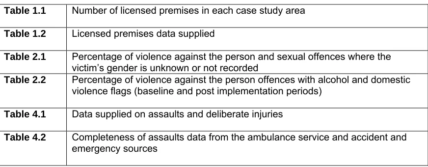
List of tables
[image:6.612.86.522.116.286.2]Table 1.1 Number of licensed premises in each case study area Table 1.2 Licensed premises datasupplied
Table2.1 Percentage of violence against the person and sexual offences where the
victim’s gender is unknown or not recorded
Table2.2 Percentage of violence against the person offences with alcohol and domestic
violence flags (baseline and post implementation periods)
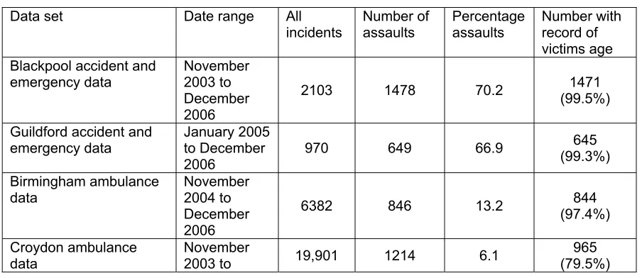
Table4.1 Data supplied on assaults and deliberate injuries
Table4.2 Completeness of assaults data from the ambulance service and accident and
List of appendices
Appendix 1 Violence against the person, criminal damage and sexual offences
Appendix 2 Calls for disorder
Appendix 3 Breakdown of codes selected for assault data from accident and emergency and
ambulance data
Appendix 4 Participant observation template Appendix 5 Topic guides
Appendix 6 Templates for semi-structured interviews (phase 2) Appendix 7 Templates for semi structured interviews (phase 3)
Appendix 8 Accident and Emergency and Ambulance data (classification codes) Appendix 9 Penalty Notices for Disorder (PNDs)
1. Introduction
The Licensing Act 2003 (LA03) hereafter referred to as the Act, came into effect on 24th
November 2005. This technical annex describes the data analysis techniques and methodologies used in a study by the University of Huddersfield to measure the impact of the Act on crime and disorder in and around licensed premises. It provides supporting material to the final report. The research, commissioned by the Home Office, examines the impact of the Act in five case study areas. These were:
• Blackpool Unitary Authority (UA);
• Birmingham City Centre (police force area F1);
• Croydon Borough;
• Guildford Borough;
• Nottingham Unitary Authority (UA).
The commissioning body selected these areas for a number of reasons. Firstly, areas were selected that spanned the broad profile of violent crime in England, taking different measures of violent crime into account and based on discussions with senior officers in police forces. All of these measures indicate that the nature and intensity of violent crime significantly differ between the chosen areas.
The selection of case study areas also provided a good mix of urban/rural area types when compared against ONS classifications of local authority districts: two cities, two smaller towns (one market town surrounded by a significantly rural population and one seasonal sea-side resort), and one London borough. A decision was made not to select any areas that were primarily rural based on Department for Environment Food and Rural Affairs (DEFRA)
classifications to avoid to undertaking focused case study work in sparsely populated rural areas, where the volume of crime data is low and it is unlikely any discernible effect on crime levels would be detected.
The final basis for choosing areas were those prepared to be involved with the evaluation and provide the crime and disorder data on a monthly basis between 2004 and 2006. Birmingham police force area F1 was used as it was agreed to supply crime data for this area.
For each area a supplementary Annex has been produced. The final report, the supplementary annexes, and this technical annex comprise a single research study. This research is part of a wider evaluation programme including a number of larger scale national measures and surveys.
Research aims
The overall aims of the research were to provide a baseline indicator of levels of crime and disorder in and around licensed premises, and to examine the impact of the Act on patterns of crime and disorder in and around licensed premises. A number of specific research questions were formulated for this research:
• What patterns of crime and disorder exist in and around licensed premises?
• What other local factors may explain the prevalence of crime and disorder in and around licensed premises?
• Does the granting of extended opening hours for licensed premises lead to a change in crime and disorder in these licensed premises?
• Have overall levels of crime and disorder within town and city centres changed following the Act?
• Has the profile of crime and disorder in and around licensed premises and associated hot spots changed in relation to new licensing hours?
• Are there any unintended consequences of the Act? For example, geographical displacement or diffusion of benefits of crime to surrounding areas.
In order to answer these questions, a number of methodologies were employed and these are described below. Often a series of methodologies have been used to answer a single research question.
Research design
There are a number of analysis methods that might be used to assess impact of the Act, although not all are applicable to an area-based evaluation of this type, for example, the use of
hypothetical comparison groups. Three area based methods were considered for this research. Only the first of these is entirely experimental in the sense that it can, if successfully conducted, control for all potential threats to validity such as maturation and selection effects. The remainder are quasi-experimental.
Randomised control trials (RCT)
Offenders or places are allocated at random either to the intervention/policy area or to a control group/control area who will either receive a different intervention/policy or treatment as usual. This approach minimises the chances that the treated and comparison groups differ in significant and important ways and that one group is biased from the outset to do better or worse. It is evident that a RCT is not a viable approach to an evaluation of a piece of legislation introduced within one jurisdiction. This is because the legislation affects the population over the same time period, meaning that the creation of control groups/areas is not possible. Thus, the strongest methodological approach to determining causality of an intervention (in this case legislation) on an outcome was not available for this specific research.
Matched pairs
In this instance, people (or areas) exposed to an intervention or policy are matched with people (or areas) given no intervention or some other intervention. The ability of this type of design to rule out threats to validity is very dependent on the closeness of the match. In other words, it is vital to control for all variables which might theoretically be expected to impact upon the outcome measure/s. Retrospective matching (where data are collected after the event) is less satisfactory than prospective matching (data are collecting before and during) but more common and less expensive. This is because the samples are matched on information contained in records rather than the evaluator making active decisions about what should be recorded and what the samples should be matched on.
Within the current evaluation it had been hoped to prospectively match premises which applied for and received extended hours with those premises which did not. Even if this had been possible (which as described below is not the case), this methodology would not have been ideal due to differences in key variables between premises which applied for extended hours and those which did not. For example, city centre pubs may be more likely to apply, and also be more likely
to experience crime and disorder. Furthermore, premises with a high level of crime and disorder in the baseline period may be refused extended hours for precisely that reason.
that data on baseline opening hours and post implementation opening hours as well as capacity limits were not routinely available (see below for more details). It was possible to obtain data on the post implementation hours applied for, but this involved considerable processing to generate usable datasets. An added difficulty here is that premises regularly may not use all of these applied hours.
Longitudinal status comparisons
Longitudinal status comparisons involves assessing an individual's (or an area’s) change over time and making inferences based upon the timing of the intervention and changes in outcome measures. It is important to note that without a comparison group, there is a possibility that changes in the outcome measure may be a consequence of factors unrelated to the intervention (for example, maturation). A comparison group can be included within this design to improve methodological rigour and ensure the assessment of other possible effects.
Longitudinal status comparisons differ from before/aftertests in that they sometimes involve multiple measurements of outcomes before and after the intervention. This single group longitudinal comparison is the closest research design to the one selected for this specific evaluation, as changes in outcomes such as crime and disorder are assessed in relation to the introduction of the Act. As noted previously, the national implementation of the policy precluded the possibility of using a comparison group, and this means that the design is unable to rule out (with adequate certainty) other threats to validity.
The selection of the methodology was based upon several factors, these largely relate to the difficulty of obtaining certain datasets as well as the difficulties of measuring a legislative change. This effectively constrains the methodological options open, and means that in interpreting the results of this research it is important to bear in mind that changes in outcome over time (such as crime) may be due to factors other than the introduction of the legislation. There are two main threats to the validity of the findings within this research
History
The effect is caused when some event, which is not the intervention of interest (e.g. increase in police numbers) takes place at the same time as the intervention/policy of interest and influences the outcome measure (for example the crime rate). There are numerous other factors which could influence crime rates and which may have occurred during the period under study. These include economic factors, other policing initiatives, sporting events, changes to police recording crime practices, introduction of SIA accredited door supervisors as well as factors such as the weather.
Regression to the mean
This is a statistical phenomenon whereby extreme scores tend to return to the mean over time, even if there is no intervention. In other words, left alone, things tend to return to normal. Such changes are often mistakenly assumed to indicate that the policy or intervention has worked. When studying time series data on crime rates, for example, it is important to recognise that year by year fluctuations may be entirely normal and not due to any particular intervention.
Research context
One of the major difficulties in conducting this piece of research is the inability to define a control area not affected by the introduction of the Act. In addition, it is difficult to isolate the impact of the Act as the geographical dispersal of licensed premises is such that there is an inter-dispersal of premises that have extended their hours of trading post implementation. One methodological step to address these problems is the use of multi level analysis.
Scale of analysis
The quantitative analysis used in this research examines crime and disorder over the baseline and post implementation periods at three geographical scales. These are:
• The macro level (aggregated data for the entire case study area).
• The meso level (aggregated data near to licensed premises).
• The micro level (data aggregated to inside or directly outside licensed premises). It should be noted that while there are advantages to using this three pronged geographical approach, some care should be taken in interpreting findings. Some potential errors of note are the Modifiable Areal Unit Problem (MAUP) and the ecological correction. These are discussed in more detail later in this report.
Timescale
This research examined two time periods, a two year baseline period before the introduction of the Act (23rd November 2003 to 23rd November 2005) and a post implementation period (24th November 2005 to 24th November 2006). This enabled a two year baseline and a full twelve months of post implementation data to be examined.
Research approach
A number of quantitative crime analysis methods were adopted for this research. The data sources used were as follows:
• Police recorded crime data (offence data).
• Police calls for service data (disorder incidents only).
• Licensed premises data.
• Accident and emergency data.
• Ambulance call out data.
• Ordnance Survey AddressPoint®.
• Ordnance Survey 1:10 000 scale raster.
• UKBORDERS digital boundaries.
• Office for National Statistics (ONS) mid-2005 population estimates1. • ACORN 2006 population estimates1.
• Penalty Notices for Disorder (PNDs)2
This quantitative crime analysis was supplemented by qualitative fieldwork which involved participant observation in the main drinking areas and inside key drinking premises, as well as semi-structured interviews with licensees, door supervisors and bar staff. These took place during
1 This was the most up to date information available that was coterminous with the case study
boundary
the baseline and post implementation periods. This mixture of analysis techniques increases the robustness of the findings.
A note on the licensed premises data
Obtaining accurate information on licensed premises was found to be more problematic than had been anticipated. Information requested included the following fields:
• Name of premise.
• Full address and postcode.
• Grid reference (easting and northing).
• Capacity.
• Trading hours before the Act (baseline period).
• Status regarding application for additional trading hours (post implementation).
• Date additional hours granted/refused (if applicable).
• Current trading hours (post implementation).
Unfortunately, initial expectations regarding the availability of this information were highly over- optimistic. There are several reasons for this discrepancy which are outlined below.
• The Inn Keeper database was used by the police to keep information on premises in four of the five case study areas. However, this system became redundant with the introduction of the Act and therefore certain information was no longer available.
• As a result of the Act, Local Authorities Licensing Authorities became responsible for
administrating licenses and this resulted in a backlog of entries that needed to be entered into a database or new electronic system.
• This backlog was primarily due to a large number of applications being submitted over a short period of time, and a general lack of resources, as all premises were required to adhere to the new licensing requirements.
• Where case study areas did provide licensed premise data, only partial and incomplete records were obtained.
• In only one area was data on former hours available.
• Only one area provided location data on licensed premises (easting and northing). In all other areas it was necessary to geo-code the licensed premises, often from partially complete address fields.
• No case study areas provided complete records relating to capacity.
• There was a lack of consistency in the information provided, and many fields were only partially completed.
Geo-coding is a process by which structured address fields that distinguish property numbers from streets, districts and unit postcodes are matched against a gazetteer to append a 12 figure Easting and Northing grid reference to each record. For this research project, the process was time consuming as it was necessary to first enhance the partial information provided on licensed premises (using internet search engines and online business addresses).
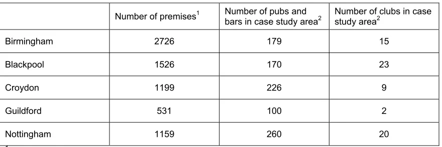
Due to the difficulties in obtaining accurate information on licensed premises, this research project only examines crime and disorder around three types of licensed premises, namely pubs, bars and night clubs. It is acknowledged that there are limitations to this as premises such as off-licences, supermarkets and restaurants are excluded.
Table 1.1 Number of licensed premises in each case study area
Number of premises1 Number of pubs and
bars in case study area2 Number of clubs in case study area2
Birmingham 2726 179 15
Blackpool 1526 170 23
Croydon 1199 226 9
Guildford 531 100 2
Nottingham 1159 260 20
1 Note this is the number of premises supplied by the licensing authority and not necessarily the
number of premises that are situated inside the case study area.
2 This includes premises with an address that could be accurately geo-coded only.
Table 1.2 Licensed premises datasupplied
Format
(note all supplied as electronic)
Address coded
Geo-Current opening hours
Former opening
hours
Extended hours
Yes/No Capacity
Premise type
Birmingham Individual records Partial X √ x x x √
Blackpool Single Database Partial X √ √ √ √ √
Croydon Individual records Partial X √ x x x x
Guildford Single Database Partial Partial √ x x x √
2. Crime
data
analysis
This section describes the different quantitative analysis techniques used to examine crime and disorder within the case study areas, particularly focusing upon areas in and around licensed premises.
Description of the data
The police recorded crime data was supplied on a regular basis by each of the five forces, to the commissioning body who, in turn, supplied the records to the research team. This data provision was separate to the compulsory Annual Data Return (ADR) that all forces are required to submit to the Home Office (HO) which is published regularly under National Statistical Protocols. Three categories of police recorded crime data were used for this research. The HO codes used to define these categories are provided in Appendix One. These were requested by the
commissioning body as they have been shown by previous HO research and analysis to be those likely to be associated with alcohol and the night-time economy. The categories examined were as follows:
• Violence against the person.
• Criminal damage.
• Sexual offences.
In addition to these categories, these data were supplied with a number of fields. Those standardised across the five case study areas examined were:
• Crime number.
• Date and time of offence (reported and committed).
• HO code (see Appendix One).
• BCU/OCU identifier.
• Offence location (full address including postcode).
• Easting and northing (grid reference).
• Modus Operandi details (short summary of offence).
• Victim’s age and gender.
Some additional fields were requested. These were ‘flags’ to indicate;
• If the offence could be attributed to a licensed premise.
• The name of the licensed premise.
• If alcohol was considered to be involved in the offence.
• If the offence was considered to be domestic violence.
Data accuracy and reliability
On receipt of data, validation procedures were conducted to identify any inconsistencies,
anomalies or missing data. Steps were then taken to cleanse the data to improve the quality and utility of the data analysis. This involved a three stage process outlined in the sections below.
Data capture and cleaning
• Standardisation of date and time fields to enable merging of files from different sources.
• Validation of location data.
• Splitting address components into separate variables (e.g. distinguishing the house number, street, town and unit post code).
• Identification and validation of extreme values.
• Identification of missing data.
Data coding
The data for each case study area was also imported into the statistical package SPSS. This enabled the generation of a number of new fields for analysis. The new fields generated included:
• Day of week.
• Month.
• Year.
• Time of day.
• Time of day interval (time of day was split into twenty four equal intervals, for example 1.00am to 1.59am, 2.00am to 2.59am and so forth).
• Baseline year 1 (24th November 2003 to 23rd November 2004).
• Baseline year 2 (24th November 2004 to 23rd November 2005).
• Post implementation (24th November 2005 to 23rd November 2006).
• Quarterly period (the data was spilt into three month periods, eight before the introduction of the Act and four after the introduction of the Act).
• Age category (0-4, 5-9,10-14,15-19,20-24 and so forth up to 80 plus).
The data were also exported into a Geographical Information System (GIS). For this research the ESRI package ArcGIS was used. This allowed for the validation of each offence’s location (easting and northing). This process is described below. It also allowed individual offences to be identified by additional location information. The first of these were concentric buffer zones, and the second was an area with a high density of licensed premises. These are both described in the GIS analysis section below.
Validation of location data
The police recorded crime data provided for this research contained a geo-reference for each individual crime offence. This was a 12 figure grid reference using the OS national grid. The coordinates for the location of offences are often referred to as the easting and northing. The grid references can then be displaced as points on a map and are used in GIS to pinpoint the precise geographical locations of offences.
Methodology
A range of methodologies were used to analyse the crime data, and often multiple methods were applied to answer the research questions outlined earlier. The methodologies used were as follows.
Distribution of offences (daily, weekly, monthly and by time of day)
For each of the three categories of crime data examined (violence against the person, sexual offences and criminal damage), exploratory analysis was carried out to examine trends in the monthly, yearly, weekly and daily crime patterns, and to consider whether the Act may have influenced these trends.
Crime rates
Monthly crime rates were calculated for each of the five case study areas. For Birmingham the case study area was the city centre (police force area F1 as this was the area data was supplied for). Here Acorn 2006 population figures were used as the case study area was not coterminous with wards used in the census. In all other case study areas, population figures from the ONS 2005 population estimates (the most up to date figures at the time of writing) were used as the ward boundaries were coterminous with the case study area boundaries.
The post implementation crime rates were calculated as a monthly rate per 10,000 persons. The baseline rates were calculated as a rate per 10,000 persons of the average monthly baseline frequencies of crime. Hence, for the post implementation period of January 2006, the baseline rate uses the average of the corresponding baseline months January 2004 and January 2005. There are limitations with using residential populations to calculate crime rates, particularly when the feature of interest is crime near to licensed premises. There are a number of potential reasons for persons to be present in public places, perhaps because of where they live (the residential population), or because they are visiting an area (for business, pleasure, for leisure purposes, for education), or for other reasons. This will also vary by time of day, and by day of week and month of year. Blackpool, for example, is a seasonal resort and its population will vary by peak and off peak seasons. Guildford, Nottingham and Birmingham all have large universities and the populations will vary during term time and holidays. However, it is extremely costly and problematic to produce population estimates for local areas based upon survey data. For this reason, the research used residential population to generate crime rates for each area. These are typically used in England and Wales crime statistics.
Percentage change
The percentage change was calculated for monthly periods between the baseline period and post implementation period. For each monthly period in the baseline period, the average count was used. Thus, the percentage change in January 2006 was the change between the crime count in January 2006, and the average crime count of January 2004 and January 2005.
Proportional change
The proportional change analysis compares data from the baseline period with the post
implementation period by time of day. To calculate proportional change the following procedure was used. For the post implementation period, the times of day of all offences were split into 24 equal intervals (midnight to 0.59am, 1.00am to 1.59am, 2.00am to 2.59 am, and so forth). For each time interval the percentage of offences was then calculated (as a percentage of all offences over the 24 hours). For the baseline period the same method was used to calculate percentage of crime by time of day interval. The proportional analysis then compares the change in the two percentage figures (baseline average and post implementation) for each time interval.
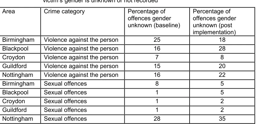
Victim profile
[image:17.612.91.515.358.563.2]The offence records contained categories for both the age and gender of the victim. However, this was not always recorded, and the percentage of unrecorded offences also varied by case study area. Table 2.1 shows the percentage of violence against the person and sexual offences where the gender is not known or not recorded for each case study area, both in the baseline and the post implementation periods. This varies between seven and 28 per cent for violence against the person and between one and 35 per cent for sexual offences. This makes comparisons between different case studies difficult. In addition, in some case study areas there was a ten per cent difference between the baseline and post implementation periods in the number of offences where the gender of the victim was unknown.
Table 2.1 Percentage of violence against the person and sexual offences where the
victim’s gender is unknown or not recorded Area Crime category Percentage of
offences gender unknown (baseline)
Percentage of offences gender unknown (post implementation) Birmingham Violence against the person 25 18 Blackpool Violence against the person 16 28 Croydon Violence against the person 7 8 Guildford Violence against the person 15 20 Nottingham Violence against the person 16 22 Birmingham Sexual offences 8 5 Blackpool Sexual offences 1 5 Croydon Sexual offences 1 2 Guildford Sexual offences 1 2 Nottingham Sexual offences 28 35
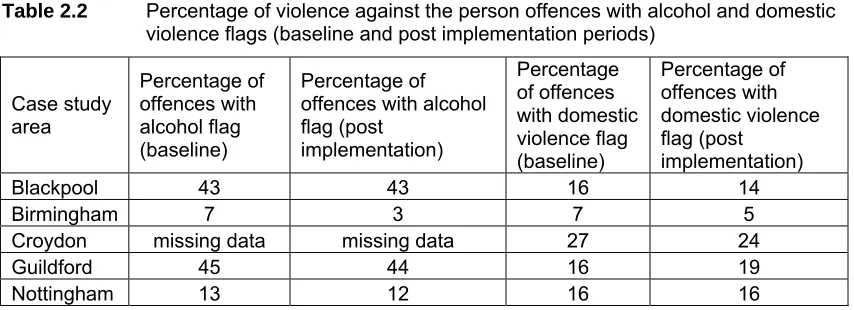
‘Alcohol’ and ‘domestic violence’ flags
The crime data contained flags for offences considered to involve alcohol or domestic violence3. These flags are subjective and were not reported consistently across the five study areas. Table 2.2 shows the percentage of violence against the person offences with alcohol and domestic violence flags for the baseline and post implementation periods. This demonstrates that there was wide variability in the use of these codes between the five police forces who supplied the data. In addition, there were differences between the percentages of offences with alcohol and domestic violence flags recorded in the baseline and post implementation periods. However, it
3 Defined by the Home office as “any violence between current and former partners in an intimate
was difficult to state with any confidence whether this change was due to the Act, or due to the way the flags were recorded.
[image:18.612.89.516.153.308.2]Three of the five forces have commented on their use of these flags and the rules they use for these. It was suggested to the authors that these flags are as accurate as possible, however, it was also acknowledged that they rely upon the subjective view of the police officer present.
Table 2.2 Percentage of violence against the person offences with alcohol and domestic
violence flags (baseline and post implementation periods)
Case study area Percentage of offences with alcohol flag (baseline) Percentage of offences with alcohol flag (post implementation) Percentage of offences with domestic violence flag (baseline) Percentage of offences with domestic violence flag (post implementation)
Blackpool 43 43 16 14
Birmingham 7 3 7 5
Croydon missing data missing data 27 24
Guildford 45 44 16 19
Nottingham 13 12 16 16
As there are difficulties in collating data with an alcohol flag, this research used time and location stamped data as an indirect measure of alcohol related crime and disorder. Thus, the time of day of incidents (particularly between 9.00pm and 5.00am) and the location of incidents (proximate to licensed premises) has been used as an indicator of such crime and disorder levels, and its change (if any) baseline between the baseline and post implementation periods.
GIS analysis
A GIS is a computerised system for the capture, storage, retrieval, analysis and visualisation of spatial data (Jones, 1997). It allows crime to be mapped over time and space, and to be cross referenced with multiple data sources, for example licensed premises and land use. The
distribution of crime in an area is not random, and the analysis of spatial patterns of crime is now a well established technique used to examine the complex interaction between crime, space and time. Within the case study areas the distribution of both licensed premises and crime is not random, and GIS enables the relationship between the two to be analysed. Furthermore, the relationship can be tracked over time, and change monitored in relation to a changing landscape (for example changes to the supply points of alcohol).
One of the benefits of GIS is that patterns of crime can be examined at different geographical scales. Hence, in addition to looking at crime over the entire case study area (macro level), crime can be examined in smaller areas within the case study area (meso level) or in precise locations such as inside or directly outside licensed premises (micro level). Changes that occur at the micro level and meso level may be masked by the overall patterns of crime in the entire study area. Thus, examining crime patterns at all three levels enables specific changes to be detected (for example changes to crime near to licensed premises).
premises. The second included areas with a cluster of licensed premises, effectively hot spots not of crime but of licensed premises, or areas with high densities of premises.
One of the advantages of GIS is that individual disaggregate data can be aggregated to various spatial units, for example police beats, census wards and buffer zones. However, it is important to note that one potential error that may arise is the modifiable areal unit problem (MAUP)
(Openshaw and Taylor, 1981). This may occur because spatial analysis can be sensitive to the definition of the units for which data are aggregated. By altering the shape and size of the boundaries used, the outcome of analysis may also be altered. To allow for this, two distinctly different methods were used to aggregate the data. The first were buffer zones - to examine proximity to licensed premises at 50 metre intervals. The second were licensed premise clusters - produced by a mathematical clustering technique to examine the cumulative effect of licensed premises.
The ecological fallacy (Brown, 1991) exists when assumptions are made that relationships that hold true for groups (based on aggregated data) will necessarily hold for individuals. One example of this is if an area with high levels of unemployment was identified as having a high number of offenders, it is assumed unemployed people are offenders. It is important not to make assumptions about an individual who lives in the area based on aggregate data about the region. The individual fallacy (Landman, 2000) is in effect the opposite of the ecological fallacy, when an assumption about a group is inferred from characteristics of an individual in that group.
By altering the unit of analysis the results of analysis can change dramatically. Hot spots or clusters of crime may occur on the global scale or at a more localised scale. Clusters of crime may be discovered at a particular location, but this will vary dependent upon whether examining at the macro, meso or micro scale. For example within an area of relatively high crime identified at the meso level, there may be smaller pockets of high and low crime areas apparent when examined at the micro scale.
Buffer zone analysis is a technique used to analyse discrete objects, for example the location of a pub or a bar, and to examine discrete areas surrounding these features. 50 metre concentric buffer zones were generated around licensed premises to produce a number of zones - the first up to 50 metres from premises, the second 50 to 100 metres, the third 100 to 150 metres, and the fourth 150 to 200 metres. This allowed crime patterns in each of these pre - defined zones to be explored and tracked over time. This analysis was used to reveal whether there were any
changes in the spatial and temporal patterns of crime near licensed premises, or if their had been any displacement of crime away from licensed premises since the introduction of the Act.
As was mentioned within the introduction to this section, licensed premises were not randomly distributed within the case study areas. Analysis of the spatial distribution of licensed premises using the Nearest Neighbour Index (NNI) revealed that there was evidence of clustering in the spatial distribution of premises. The nearest neighbour index (NNI) figure is a statistical test used to validate that there is evidence of hotspots and that the data are clustered. A value of less than one (as found for both violence against the person and criminal damage) indicates the data are clustered, and that these hot spot methods are appropriate. The Z score is a measure of confidence in the NNI, the more negative this is the more confidence can be placed in the findings.
Hot spot analysis
Areas with a high concentration of crime are often described as hot spots (Eck et al, 2005). There
are a number of theories around why crime is concentrated in particular localities, and these may be around individual points or groups of points, around individual streets or groups of streets, or around particular neighbourhoods. Hot spot analysis focuses upon examining why areas have above average numbers of crime offences, and hot spots are often cross referenced with the physical infrastructure and social conditions of an area to attempt to explain such concentrations. Hot spots may form due to repeat victimisation, near repeat victimisation, or the presence of risky facilities (Clarke and Eck, 2005). Licensed premises could be described as a risky facility for crime, and hot spots may form around these. Thus, hot spot analysis was used to explore whether the location of hot spots in the case study areas had shifted since the introduction of the Act.
It is important to test for the presence or absence of hot spots in crime data before running hot spot analysis, and the test used for this was again the NNI. In all case study areas there was evidence of clustering in the data and two different types of hot spot methods were used in this analysis. Nearest Neighbour Hierarchical Clustering was the first technique used. The software used for this was CrimeStat 3 (a free software package available online4). This technique uses
nearest neighbour analysis of points (licensed premises) and only points that are closer than expected under spatial randomness are identified. A set of ellipses are produced called first order ellipses. Grouping these clusters using this method can then generate second order clusters, and this process is repeated until all points fall into a single cluster (Levine, 2002). For the purposes of visualisation, second order clusters are displayed in the figures used within this research (see individual case study area annexes). Visually comparison suggested this were the most appropriate level to use.
It is important to note the limitations of the NNHC analysis. It is sensitive to some parameter settings, and may fail to represent actual spatial distributions of data (clusters of bars and crime do not naturally form ellipses). However its purpose is to identify areas where there are clusters of premises within which crime can be measured. An alternative for future research may be to use the Gi* statistic. However, although this can identify spatial significance it does not identify spatially significant change. For more information the reader is referred to the CrimeStatmanual (Levine 2004) and a recent pubilication by Eck et al., which detail hot spot techniques in detail.
For this research, the baseline crime data and the post implementation crime data were used to generate baseline and post implementation hot spots. Hot spots were produced for violence against the person and criminal damage. Due to the small numbers, hot spots of sexual offences were not generated. The advantage of these ellipses is that they identify areas that are not geographically defined except by the extent of the cluster. They are a product of the location of crime points and do not reflect the layout of the underlying area. They allow a visual examination of the location of crime hot spots that can be mapped against the location of licensed premises. As they are based upon a minimum of 12 months of crime data, they represent areas that can be considered fairly stable. For this analysis, differences in hot spots by time of day were not explored, as interpolation methods were thought to be most appropriate.
The second hot spot analysis technique employed was kernel density estimation (KDE) interpolation, again using CrimeStat 3. Interpolation aggregates points within a user specified search radius and smoothes the data into a continuous surface. As crime data is discrete to individual points, an appropriate method suggested for this is quartic kernel density interpolation (Eck et al, 2003). This creates a grid over the crime data points. A weight is assigned to each
point within a user defined bandwidth and within this density points are calculated for each point using mathematic functions. Grid cell values are then calculated by summing the value for all
circle surfaces generated. It allows a continuous surface to be generated that is based upon calculations at all locations as opposed to alternative methods that discard some locations. This continuous surface allows for crime clusters to be easily interpreted and accurately reflects the spatial distribution of the data. For more information on this technique see Eck et al (2003) and
Levine (2002).
For this research, quartic KDE interpolation hot spot maps were generated for both violence against the person and criminal damage. It is also known that hot spots vary by time of day. Based upon the results of the proportional time of day analysis, and as these were though to be most influenced by the Licensing Act, four time intervals were examined (all two hours) for both the baseline period and post implementation period. These were as follows:
• 9.00pm to 10.59pm.
• 11.00pm to 0.59am.
• 1.00am to 2.59am.
• 3.00am to 4.59am.
Crime ratios
Crime ratios are used to express how much crime in an area of interest occurs in respect to a wider reference area. For the purposes of this research, the areas of interest used were the cluster areas of licensed premises (areas with a high density of licensed premises). The crime ratio is the amount of crime in the cluster area divided by the amount of crime in the remainder of the case study area. This was examined over twelve quarterly periods, eight before the Act and four after the Act. Quarterly periods are commonly used to analyse crime ratios. A crime ratio of 1.0 implies that the cluster area and the reference area (remainder of the study area) each contribute the same proportion of crime to the study area. A crime ratio of 0.5 implies the cluster area contributes one third of the study area’s crime, and a ratio of 2.0 suggests that the cluster area accounts for two thirds of the case study area’s crime. This analysis determines whether the cluster area (high density of licensed premises) is accounting for a greater proportion of the case study area’s crime over time.
Resource Targeting Tables
It has been suggested that licensed premises may be risky facilities, and it is also known that crime tends to be concentrated both in time and place. A Resource Targeting Table (RTT) is an innovative technique for identifying how much of a problem (crime) is concentrated in varying proportions of licensed premises. For the purpose of this analysis, violence against the person offences were examined, and the licensed premise flag was used to assign individual crime offences to an individual licensed premise. Criminal damage was not examined in this way as the data structure did not flag premises against damage offences. This may be when a violence against the person offence occurred inside or directly outside (in the vicinity of) a particular premise. It is used to attribute violence against the person offences to licensed premises. It should be noted that there are a number of limitations to this analysis. As there is no causal link between the premise and the offence, it is possible that the victim and offender were outside a premise when the offence occurred, but only one or neither of these had been inside the premise in the events leading up to the offence. Furthermore, a premise may be exhibiting good practice by refusing entry to an intoxicated person, yet this person may then cause an offence outside the premise (linking the offence to that premise). Despite the limitations, this technique is useful in determining how concentrated violence against the person is amongst licensed premises, both for targeting resource prevention and monitoring how the Act has influenced this concentration over time. This technique allows useful questions to be posed including:
• How many premises contribute to 25%, 50% or 75% of the offences?
• How has this changed since the introduction of the Act (how many premises have remained in the Top 15 for example)?
It should be noted that there are limitations with the RTT analysis. The format of the data makes it difficult to attribute an offence to an actual premise, thus it refers to offences that occurred inside to directly outside a premise (linked by premise name in the recorded crime data). However offences may occur on street corners adjacent to a number of pubs, or a door security person may refuse entry to an intoxicated person who may cause an offence. Thus care should be taken when attributing offences to an individual premise. Furthermore, these take no account of the size of a premise, its capacity, or the number of hours it remains open. However, this technique is very important for measuring risk, as the volume of offences does relate directly to police the level of policing required at a particular location. Moreover, a premise may have been closed down for part of the year. If this still appears in the top 15 list, then this heightens its risk as it may not have been open for as many months as a premise with fewer offences. However it is acknowledged that if a premise with a small capacity has a relatively high number of offences (in relation to its size) then this may be missed using this analysis. It is suggested this analysis could also be included in any future analysis.
Additional hours used (sample premises visited)
One of the difficulties faced in this research was obtaining accurate information on changes in licensed premises’ opening hours baseline to post implementation. Indeed, even where data was obtained on baseline trading hours and post implementation hours applied for, this did not equate to actual additional hours used. The qualitative research and other research conducted in the case study areas (see Cragg Ross Dawson study for example) suggested although premises applied for additional hours, they typically did not use all the hours entitled to them. To examine this further, the qualitative fieldwork was used to gather information on additional hours applied for (from licensees and licensing authorities) as well as additional hours used on average, per week. This was undertaken at those premises visited during phase three of the fieldwork, as detailed later in this report.
The number of additional hours used per week was then compared with the number of additional
hours applied for per week. This gave an average percentage of additional hours used by premises in each of the case study areas. It should be noted that this figure is based on a small sample of less than fifteen premises in some study areas.
In addition, the additional hours used by premises each week was grouped into three categories - none, low and high. The total number of violence against the person offences at each of these premises were then summed for each of the three additional hours categories. This gave the total number of offences for each grouping, for both the baseline and post implementation periods. For each category, the average number of offences in the baseline periods and post implementation periods were calculated. The changes in volume and in the proportion of offences in each category were then calculated, to compare base line and post implementation periods by number of additional hours used. Unfortunately because of the data structures, it is difficult to link
Additional hours applied for (estimated for all premises)
In addition to examining the additional hours used at the sample of premises visited during the
fieldwork, additional hours applied for per week were estimated for all premises in the study area.
It proved to be difficult to obtain data on former trading hours (during the baseline period). For this reason, the researchers estimated these to be 11.00pm for pubs and 2.00am for night clubs. The data on current hours appliedfor(not necessarily those used) were then used to generate
additional hours applied for per week for all premises in each case study area.
These hours were then grouped into three classifications - no additional hours, low additional hours and high additional hours. For each of these three groupings, the number of violence against the person offences at each of the premises were summed to give a total number of offences in each group, for both the baseline and post implementation periods. The changes in volume and in the proportion of offences in each category were then calculated, to compare base line and post implementation periods by number of additional hours applied for. Again because of the data structures, and for the reasons stated above, it is difficult to link offences by time of day and day of week.
Limitations and analysis not considered
There were a number of analyses that were not considered appropriate for this research. The analysis of the sexual offences data was only carried out at the macro level, as numbers were too small to perform meaningful meso and micro level analysis.
Criminal damage offences often have a date/time range recorded in the crime record that refers to when the crime occurred. The exact time is often not known because the offence could have been caused to property and not been brought to the attention of the owner until some later point. Temporal analysis of this type of crime data often uses a weighted (also referred to as an aoristic) approach. However, preliminary analysis of this time range field suggested this would not be appropriate here (see Appendix 11). The analysis splits the crime data into one hour intervals. 40 per cent of all offence records did not contain a ‘to field’, and, almost 75 per cent of all offence records either had a ‘to time’ field that occurred within one hour of the ‘from time’, or did not contain a ‘to time’. Thus, use of the ‘from time’ field was considered the most appropriate for the purposes of this research. Thus the proportional and time of day analysis is based on the ‘from’ time of day field only.
Due to the difficulties in obtaining accurate data on the baseline hours of licensed premises, and accurate information on whether premises had extended and/or used extended hours during the post implementation period, it was not possible to use the matched comparison analysis as originally intended for the research. Furthermore, difficulties in linking the violence against the person offence data to individual premises precluded the use of this matched pair analysis. The difficulties in constructing this analysis have enabled yearly breakdowns of these offences, but resource constraints have restricted further analysis by weekends and night-time offences. There are a number of potential errors that arise in the crime analysis. The first of these errors is due to the under-reporting of crime data (Walker, Kershaw and Nicholas, 2006). The 2005/2006 British Crime Survey suggests that approximately 42 per cent of comparable crimes are reported, although this varies by crime type. For violent crime this figure is approximately 68 per cent, for common assault this figure is much lower (35%). The under-reporting of crime is well
police may deter potential offenders and actually reduce crime. Thus, A&E and ambulance call out data was used to supplement this crime analysis.
When examining change over time however, there is no reason to suggest (and the qualitative fieldwork supports the likelihood) that the reporting of crime data has not changed between the baseline and post implementation periods. Thus, whilst the under-reporting of crime data should be acknowledged, it is unlikely to explain any changes found in crime patterns between the baseline and post implementation periods. However, as stated above, there are some changes to the classifications of ‘serious violence against the person offences. Recent changes in the National Crime recording Standards (NCRS) influenced how Threats or Conspiracy to Murder are recorded (this was introduced in February 2005 (Walker et al, 2006) and recent changes aimed at over-preventing of less serious threats and is likely to have contributed to falls in no injury
violence. As a result of this the violence against the person offence data was separated into more and less serious offences. However, because only three per cent of offences were classified as ‘more serious’, only annual comparisons were examined. The results of this are analysis are shown in the Final report, and the methodology used described in the supplementary analysis section of this technical annex.
The recorded crime data will also be influenced by seasonality (Hird and Ruparel, 2007) as it is affected by short-term effects associated with the time of year. These short term effects can obscure longer term trends in the data, and it is important to consider these when interpreting any change observed. Violent assaults and sexual offences, for example, are typically high during the summer months and lower during the winter. Criminal damage tends to have peaks in the spring and autumn, with a slight fall in the summer. Thus, it is important to consider longer term change over a twelve month or longer time period. In addition to seasonal factors, other influences on the recorded crime data may include music festivals, carnivals, and bank holidays, or demonstrations and riots which may vary by location and time of year. For this reason, the crime data are
examined over a three year period where possible.
Another potential influence on the crime analysis is the influence of police operations and activity in the case study areas. Alcohol Misuse Enforcement Campaigns (AMECs)5 involve short (typically eight week) police-led operations to tackle alcohol-related crime and disorder. AMEC was spearheaded by the Home Office Police and Crime Strategy Unit (PCSU) and the
Association of Chief Police Officers (ACPO) and was designed to send a clear message that alcohol-related violence or underage sales/drinking would not be tolerated. The first campaign involved 92 of the 255 Basic Command Units (BCUs) across the country, and 46 trading standards departments, focusing energies and activities around weekends and bank holidays – the busiest time for alcohol-related offences. These were ongoing during the time period analysed.
Furthermore, in some of the case study areas, including Nottingham, the Tackling Violent Crime Programmes (TVCP6) were in operation. The timing of both AMECs and TVCPs are highlighted
in the individual case study annexes.
Finally, at the outset it had been hoped to incorporate additional contextual information into the analysis. Although there is an abundance of residential neighbourhood classifications, such as ACORN that is used in the British Crime Survey, no equivalent classification exists for non residential areas. There is a clear need for such a classification to be developed, especially to inform studies that seek to identify and explain changes in crime in areas associated with the night-time economy. If such a classification were available for the whole country this would complement existing residential neighbourhood typologies commonly referred to as Geodemographic classifications.
5http://police.homeoffice.gov.uk/operational-policing/crime-disorder/alcohol-misuse 6http://www.crime-reduction.gov.uk/tvcp/tvcp03.htm and
In the absence of a non residential land use classification, individual components of relevant land use would have to be selected and captured within a GIS. The most relevant would have been alcohol supply points other than pubs and clubs (restaurants, off licenses, supermarkets), major transport routes, taxi ranks and late night shops/ fast food outlets. Given the difficulties in just being able to capture data on pubs and clubs, extending the analysis to capture land use components was deemed infeasible.
In the present study some idea of land use is provided by data derived from the GIS analysis on the density of pubs and nightclubs found in demarcated town centres. Density in this sense is represented by the inter-pub distances expressed in metres in areas of concentrated drinking. These are compared with pub densities in areas outside of the main pub clusters in each of the case study areas. The ratio between the two (i.e. the average distance between pubs in the main drinking circuits divided that between pubs in the rest of the town) gives some idea of the greater concentration of establishments in the main areas of interest.
3. Disorder data analysis
This section of the annex describes the different quantitative analysis techniques used to
examine disorder within the case study areas, particularly focusing upon the areas in and around licensed premises.
Description of the data
Police calls for service records (disorder incidents only) were supplied for all five case study areas. These are logs of calls made by the public for police assistance. The following fields were supplied for all five areas:
• Date of incident.
• Time of incident.
• Incident code7.
• Incident location (full address including postcode).
• Easting and northing (grid reference).
For each of the five case study areas, disorder codes were extracted from the calls data
(Appendix Two). It should be noted that the codes used by each of the five police areas were not standardised across each area, therefore, care should be taken when comparing results between the five areas.
Data accuracy and reliability
On receipt of data, validation procedures were conducted to identify any inconsistencies,
anomalies or missing data. Steps were then taken to cleanse the data to improve the quality and utility of the data analysis. This involved a three stage process which was identical to the crime data validation.
Data capture and cleaning
The incident data was captured and cleaned using the same methods as the crime data
Data coding
The data for each case study area was also imported into a statistical package SPSS. This enabled the generation of a number of new fields for analysis. These were identical to those for crime data except there was no age category supplied with the incident data.
The data was also exported into a GIS to validate the incidents location. The procedure was identical to that of crime data.
Validation of location data
The methods used to test the accuracy of the location of calls data was identical to the procedure used for the crime data. For each of the five case study areas, the research team were satisfied that the accuracy of the police geo-coded disorder data was of a high quality and was suitable for the purposes of this research. It is important to note that in one area, Croydon, the data was not supplied by one metre grid references (easting and northing) but by 100 metre grid squares. This
impacted slightly upon the analysis undertaken here, and this is described in more detail within that separate annex.
Methodologies
A range of methodologies were used to analyse the disorder data. These are outlined below.
Distribution of incidents (daily, weekly, monthly and by time of day)
Exploratory analysis was carried out to examine trends in the monthly, yearly, weekly and daily disorder patterns, and to consider whether the Act may have influenced these trends.
Incident rates
Monthly incident rates were calculated for each of the five case study areas. The population estimates used in each area were the same as those used to analyse the crime data. The post implementation rates were calculated as a monthly rate per 10,000 persons. The baseline rates were calculated as a rate per 10,000 persons of the average monthly baseline frequencies of disorder incidents. Hence, for the post implementation period of January 2006, the baseline rate uses the average of the corresponding baseline months January 2004 and January 2005.
Percentage change
The percentage change was calculated for monthly periods between the baseline period and post implementation period. For each monthly period in the baseline period, the average count was used. Thus, the percentage change in January 2006 was the change between the incidents count in January 2006, and the average incident count of January 2004 and January 2005.
The average percentage change was also calculated for time of day. Incident counts for each year were divided by time of day (into twenty-four one hour time intervals). The baseline periods were the time periods 24th November 2003 to 23rd November 2004 and 24th November 2004 to 23rd November 2005. The post implementation period was (24th November 2005 to 23rd
November 2006). The average frequency was used for the baseline period.
Proportional change
The proportional change analysis compares data from the baseline period with the post implementation period by time of day. For both the baseline periods and post implementation periods incident counts by time of day (categorised into twenty-four one hour intervals) were used to calculate the percentage of crime in the baseline and post implementation periods by each of the twenty-four time periods. The proportional change figure relates to the percentage point change between the baseline and post implementation periods.
GIS analysis
As with the crime data, spatial analysis of the disorder data was used for this research. Again, buffer zones were used to examine calls for disorder in proximity to licensed premises, and cluster areas of licensed premises were generated to examine the cumulative impact of premises on disorder in areas with high densities of licensed premises.
this reason, the margin of error of using 50m buffer zones precludes their use. For all other areas 50 metre buffer zones were used following the same procedure as used in the analysis of the crime data.
Incident ratios
Calls for disorder ratios were carried out using the same process as that outlined within the crime section, however, crimes were replaced with calls for disorder data.
Limitations and analysis not considered
The calls for disorder data did not contain fields for age and gender, thus victim profiles were not examined. They also did not contain licensed premise, domestic violence and alcohol flags, thus no analysis of this type could be undertaken. Again time and location data were used as an indirect measure of alcohol related disorder. The location of calls for disorder data was shown (running the analysis using a sample of data from some of the case study areas) to be similar to the criminal damage recorded crime data, thus hot spots of disorder were not generated. Another factor in not examining hot spots of disorder were that in Croydon this analysis was not possible, as the data was located by 100m grids (not individual points).
Care should be exercised in interpreting the calls for disorder records, because they do not reflect actual crimes. There may be multiple calls relating to one incident (although steps were taken to identify duplicate incidents in the data and remove them), thus the disorder data may be subject to over-reporting. The data may also be subject to under-reporting for similar reasons to that of recorded crime data.
Finally, the calls for service data was not standardised across the five study areas, as, unlike the recorded crime data, it is not subject to national reporting standards. This is an important
consideration when comparing the five case study areas. In addition, in Nottingham, there was a change in the classification of codes used for all calls for service types during the baseline period, which impacted upon the analysis in that there were only eight months of comparable data baseline and post implementation. In Blackpool, although new codes for disorder were introduced, these were comparable over the time period under consideration.
It is important to the disorder data for Nottingham and Guildford. In Nottingham there was a change in the classification codes used, and this change to the recording standards directly influence the number of incidents classed as disorder. This change occurred in March 2005, and as a result of this, there is not a comparison of two years of baseline data with one year of post implementation data. Instead, the analysis used an eight month baseline period (April 2005 to November 2005) and an eight month post implementation period (April 2006 to November 2006). This makes the findings less robust than the other case study areas, but this analysis is not affected by the change in codes. Using all the baseline data over the two year period would not be examining comparable datasets.
4. Health data analysis
For each of the five case study areas, data was requested on assaults and deliberate injuries from both the ambulance service, and accident and emergency departments of local hospitals. This data is used to supplement the information provided on violence against the person from police recorded crime records. The methods used to clean and validate, and then analyse this data are now described in more detail below.
Requested data
The commissioning body requested data for all five case study areas.
The A&E data and the ambulance data was used to supplement the violence against the person analysis, as it provided further information on assaults. The use of this data enables an
assessment to be made of overall levels of alcohol-related attendances (e.g. alcohol poisoning etc) and whether there was any change following the introduction of the Licensing Act. One of the advantages of using this ‘health’ data is that violence against the person (particularly more serious offences) may be reflected here. Combining health and crime data on violence and assaults in this way increases the robustness of the findings.
Data was requested by the commissioning body from one hospital A&E department per case study area. The hospital selected (if there was more than one) was the one that was most likely to receive attendances/admissions from the city centre. Data was requested for attendances on weekend nights (defined as 10.00pm Friday to 5.00am Saturday and 10.00pm Saturday to 5.00am Sunday), for those people aged between 17 and 35 years, for all presenting symptoms. It was decided to limit to data collection to these specific days, times and ages following a
discussion of the commissioning body with Professor Jonathan Shepherd, who assured the commissioning body that these factors would provide a good proxy measure of alcohol-related attendances.
Data was requested for all presenting symptoms as Prof. Shepherd8 highlighted that all A&E
departments have slightly different recording systems and not all departments routinely record whether the patient was drunk/had consumed alcohol prior to attending or whether an injury was the result of an assault or an accident. The following data was requested:
• Age of patient
• Sex of patient
• Date of attendance
• Time of attendance
Additionally, it was requested that attendances related to assault were flagged (if this was possible given the individual recording systems).
Ambulance data were requested from one ambulance station per case study area. The station selected (if there was more than one) was the one that was most likely to receive call-outs from the city centre. The requested data was for call-outs on weekend nights (defined as above), for those people aged between 17 and 35 years, for all presenting symptoms. The rationale for this is the same as the A&E data.
A summary of the classifications of incidents provided for each case study area are provided in appendix eight.
Description of the data
It was not possible to obtain both accident and emergency data and ambulance data for all five case study areas. Thus, of the data that was received, the following data sets were considered suitable for the purposes of this research.
Table 4.1 Data supplied on assaults and deliberate injuries
Case study area Ambulance data Accident and emergency data
Blackpool √
Birmingham √
Croydon √
Guildford √
Nottingham √ √
For each of the five case study areas, the following fields were supplied:
• Date of incident.
• Time of incident.
• Incident type9. • Age of victim.
• Gender of victim.
It is important to note that the incident types are not standardised across all five areas, thus care should be exercised when making comparisons between the five areas. Extracted codes are shown in Appendix Three.