A new and general importance sampling technique for the estimation of bit error rates in digital communication systems

ANew

and

General Importance

Sampling

Technique for the

Estimation of Bit Error Rates

in

Digital COInmunication Systems

Mihail Devetsikiotis

Center for Communications and Signal Processing

Department

of Electrical and Computer Engineering

North Carolina State University

Abstract

DEVETSIKIOTIS-HADJINICOLAOU, MIHAIL. A New and General Importance

Sampling Technique for the Estimation of Bit Error Ratesin Digital Communication Systems. (Under the supervision of Dr.

J.

Keith Townsend)

Importance Sampling

(IS)

is recognized as a potentially powerful method for re-ducing runtimes when estimating the Bit Error Rate (BER) of digital

communica-tion systems using Monte Carlo simulacommunica-tion. The key to its effective implementacommunica-tion,

however,is the choice of appropriate biasing parameters. Inthe past, analytical

min-imization of the variance of the ISestimator with respect to the biasing parameters

has only led to solutions for systems which the BER could be found analytically. We

present here a new technique for finding a near-optimal set of biasing parameters for

the translation biasing scheme. The near-optimal translation values can be deter-mined from repetitive, very short simulation runs by exploiting a theoretically

justi-fiable relationship between the BER estimate and the amount of translation. Only

mild assumptions are required of the noise distribution and system. Moreover, we extended the standard translation techniques tocover IiDgle-lided noise distributions by proposing a claa. of "quasi-linear" biasing schemes. Experimentalreault. indicate

that, uing the technique presented here, improvement factors of up

to

eiPt orders

Acknowledgements

Contents

List ofFigures

List ofTables

1 Introduction

1.1 Statement of the Problem 1.2 Background . . . . 1.3 Summary and Perspective

2 Model Description and Definitions 2.1 Model Description . .

2.2 Probability of Error . . 2.3 Me a.nd IS Estimators

.

.

. . . . .

.

. . . .

v vii 1 1 2 6 8 8 10 12

3 Locating Near-Optimal IS Parameters 1 7

3.1 O v e r v i e w . . . 17 3.2 Memoryless System . . . 17 3.3 System with Memory: Direction of Biasing . . . 23

3.4 Nonlinear Systems 28

3.5 System with Memory: Effects of Over- and Undertranslation . . . 35 3.6 Proposed method . . . 41

3.7 Summary 44

4 Importance Sampling for Single-Sided DistributioDS 46 4.1 Backgr'ormd . . . · · · . . . •. 46

4.2 Importance Sampling Schemes . . . 49

I) Experimental Re8ults &7

5.1 Simulation Set-up . . . 57 5.2 Linear Systems . . . 58

5.3 Nonlinear Systems 64

5.4

DiaCUSDOD...

67

6

Conclusions

89

List of Figures

2.1 Model for baseband digital communicatiolll 8Y8tem •• • • • • • • •. 8

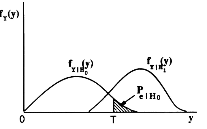
2.2 Probability distributions of }J. under H_o and HI hypotheses. The

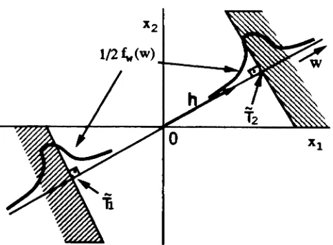
shaded &rea beyond the threshold T corresponds to the probability of error under Ho. · • . . • • • • . • • . • . . • • • . . • • . . . •• 11 2.3 Original and biased pdf's, important region Ox, and weight function

wx(z) · · · · . · · . · · . · . . . .. 14

3.1 Memoryless case: schematic illustration of underestimation proof, part 1 20 3.2 Memoryless case: schematic illustration of underestimation proof, part 2 21

3.3 A 3-dimensional input noise space with an impulse response h, a

bias-ing direction d and a decision surface

S . . . ..

24

3.4 Linear system: a 2-dimensional illustration of an impulse response h,

a biasing direction d and a decision surface (hyperplane perpendicular to h) . . . .. 26

3.5 Discrete nonlinear system model based on a cascade of a linear system with memory and an instantaneous nonlinearity . . . .. 29

3.6 An example of the mapping induced by an instantaneous nonlinearity 31

3.7 A 2-dimensional illustration of the mapping of important regions for a

nonlinear system 32

3.8 Mapping of the important region when the nonlinearity is monotonic

(in

creasin.g) 32

3.9 Input space and important regiOJUI when Ow= {1O : 10

<

1'1 or 10

>

T

2} 33

3.10 Input space and important regions when Ow

=

{1O : 1'1

>

10

>

T

2} •• 34 3.11 Syltem with memory: schematic illustration of underestimation proof,

put 1 38

3.12 Systemwith memory: schematic illustration ofunderestimation proof,

put 2 • • • • • • • • • • • • • • • • • • • • • • • • • • • • • • • • • • • 39

4.1 The WMC density distribution for three input levels (optical power)

PI

<

P2

<

PI: PI

=

-52dBm, PI

=

-46dBm and PI

=

-43dBm.

The APD characteristics were: G

=

25, Ie

=

0.8, 'I

=

0.8 and I1t = 8.92 X 10-10 • • • • • • • • • • • • • • • • • • • • • • • • • • • • • • • • 49

4.2 Three different quasi-linear biasing .chemes: (a) Tranalation with uni-form correction(b) Tranalation with "mirror-image" correction (c)

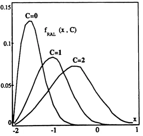
Bi-uing by increasing the input level . . • . . . • . . •. 51 4.3 Nonlinear transformation ("quasi-linear" biuiDs) ofa random variable 52 4.4 Quasi-linear biasing applied to a Rayleigh distribution, for b

=

0.3,

Ztaift

=

-2.0, Q

=

0.5 and

0

=

0, 1, 2 . . . .. 52

4.5 Quasi-linear biasing applied to a WMC distribution, for

X

= 696.59,

o

=

595.92, 6

=

1.23,Q = 60 and C

=

0, 1500, 3500 . . . •. 53 5.1 Impulse responses of the two linear, time-invariant filters that were

used in the experiments 58

5.2 Linear system: Curve of

P

e VB. the translation amount C, for the Gaussian distribution, where Pe ~ 10-10, memory length M = 24 and realization numberj

=

o. . . ..

59 5.3 Linear system: Curve of

P

_e vs. the translation amount 0, for the

Rayleigh distribution, where Pe ~ 10-10_{, memory length M}

=

_{40 and} rea1ization numberj

=

4. . . 60

5.4 Linear system: Curve of

P

e vs. the translation amount 0, for the ATE distribution, where Pe ~ 10-8, memory length M

=

40 and rea1ization number j

=

9. . . 60

5.5 Linear system: Curve of

P

e vs. the translation amount C, for the WMC distribution, where Pe ~ 10-7, memory length M

=

40 and realization numberj = 3. . . 61 5.6 Impulse responses of the two linear filters that were used as parts of

the nonlinear models . . . 64 5.7 Instantaneous nonlinearity used in the simulations . . . 65 5.8 Nonlinear system: Curve of

P.

vs. the tranalation amount 0, for the

Gaussian distribution, where p. ~ 10-1_{, memory length}

M

_{= 40 and}

realization number;

=

5. . . • . • . . . .• 66 5.9 Nonlinear Iystem: Curve of

P.

VB. the tr&llBlation amount 0, for the

List of

Tables

5.1 Estimated probabilities of error and improvement factors over

Me

sim-ulation: linear system. . . 62 5.2 Approximate runtimes in seconds, for the experimental simulations:

linear system 62

5.3 Estimated probabilities of error and improvement factors over

Me

sim-ulation: nonlinear system. . . .. 67 5.4 Approximate runtimes in seconds, for the experimental simulations:

1

Introduction

1.1

Statement of the Problem

The probability of an error (or Bit Error Rate, BER) is the most commonly used measure of performance of digital communication systems. Various studies have

ad-dressed the problem of calculating the BER based on specific assumptions about the

system and the random disturbances (noise or interference) involved [1, 2, 3]. Very

often, however, the complexity of digital communications systems makes the

analyt-ical evaluation of the error probability very difficult. In fact, for systems other than

the standard linear system with additive white Gaussian noise, analytical evaluation

of the BER is virtually impossible unless restrictive assumptions are used.

Both numerical and simulation-based methods have been proposed to overcome

this difficulty. One of the methods often used to obtain an estimate of the BER of

a systemiI Monte Carlo (MC) simulation. However, the Dumberof MC 111IlI needed

to estimate very low probabilities of error is extremely large, making the ue of

Me

simulation impractical.

Among the various techniques that have been proposed for reducing run lengths

of

Me

simulation, Importance Sampling (IS) techniquel have attracted signifiCUlt

events" , i.e., errors, that occur per simulation run by modifying the statistical

prop-erties of the noise process involved. This is gener&1ly referred to u "biasing" of the noise process. The arlifici&1ly increased error count is then corrected or "unbiased". Under the proper conditions, the above can reault in a significant reduction of the

eltimator variance or, equivalently,in significant reduction of therequiredsimulation

length.

We provide in this work a new technique for finding nea.r-optimal parameter

set-tings for IS that can be used for the efficient estimation of the BER of digital

commu-nication systems. The significance of this technique is that it is simple and general,

that is, it does not require most of the assumptions used in previous work (e.g., linear

system and/or normally distributed noise).

1.2

Background

IS is a statistical technique known by simulation practitionen for quite a while [4,

5].

However, its potential usefulness in the analysis of communication systems has been

explored only recently.

A first attempt to apply IS to the estimation of the BER of a digital

commu-nication system was presented by P. Balaban in [6]. The author proposed using IS

to reduce the runtime of

Me

simulation of Shot-noise-limited fiberguide repeaters

with an Avalanche Photodiode Detector (APD). Some fundamental concepts of IS

like "important regions" and relationships between input and output weishtl were

diacuued.

However, the practical lipificance of that work was limited by the fact

that the problem of handling Intersymbol Interference (lSI) due to

IYItem

memory

The first detailed examination of biasing and unbiasing procedures for IS and

the effects of Iystem memory and lSI was provided by K. S. Shanmugan &Ild P.

Balaban in [7]. In this paper the authors introduced the fundamental theoretical

upect. ofISwith respect to a baseband digital communication IYltem with memory.

Alsuming additive Gaussian noise, they proposed &biuing scheme that was bued on

multiplying each noise random deviate by an appropriately chosen .calar collltant,

therefore increasing the noise variance by the same factor. The ICalar constant used

was optimal for each case, in the sense that it was chosen to maximize the runtime savings over

Me

simulation. The effects of system memory length and its approximate

identification on the mean and the variance of the ISestimator were also discussed.

Finally, simulation results showing substantial savings over

Me

simulation were given.

Two of the earliest papers examining the theoretical aspects of IS and its

appli-cation to the analysis of communiappli-cation and radar systems were [8] and [9]. R. L.

Mitchell in [8] explored some of the theoretical aspects of MC simulation and IS,

and presented an extensive series of examples involving one- and multi-dimensional

probability distributions, whereISwas shown to offer significant advantages over

con-ventional MC simulation. G. W. Lank in [9] presented a detailed and mathematically

rigorous description of IS and its application to the estimation of the probability

of rare events. He developed conditions {or the IS approach to be valid and, more

importantly, to improve the efficiency of the limulation. Moreover, he preeented

bounds on the statistics of the ISestimator and studied the uymptotic behavior of

the improvement factor. Experimental result••howed the great potential for runtime

savings offered by IS.Both authon above, emphasizedmostlythe uaefulnell of ISin

radar applications and, like the authon in [7], adopted theISscheme where the noise

M. C.Jeruchimin [10] gave, among otherl, a complete description of the statistical

properties of the ISestimator and outlined the biasing/unbiasing proceduresused in

IS.

The same author in [11] extended the analy.u of IS to include multihop linb

and addressed the dectl ofphue and timing edimation on the performance of IS

techniques.

Q.W. Wang and V. K. Bha.rgaft in [12] gave a more general theoretical description

of IS in a different notation, provided useful insight in some practical upeds of

IS, and, based on the - trivial but impractical - global optimal biasing strategy,

proposed a heuristic scheme that dealt with the difficulties induced by the insufficient

knowledge about the system.

A basic disadvantage of biasing by increasing the variance of the noise [7, 9, 11]

is the significant reduction of its efficiency as the memory of the system increases. In

fact, it seems that increased system memory generally tends to reduce the

improve-ment induced by any IS scheme. B. R. Davis in [13], proposed a method to reduce

the dimensionality of the problem to unity so that the negative effects of memory

would be eliminated. Although theoretically this method could be 118ed {or a large

variety of systems and noise distributions, it seems that, for practical purposes, its

application islimited to linear systems with additive Gaussian noise.

In

[14]

P. M. Hahn and M. C. Jeruchimexamined the application of IS to Iystems

with more than one input noise processes, determined the dects of the truncation of

system memory on theISestimator and analyzed extensively the cue where the noise

is Gaussian, bued on new concepti like the STC (SYltem Threshold Charaderistic)

and the SBC (SYltem BER Characteristic). They Ihowed that, for a linearIJltem

they proposed 1lIing .tatistical regresliOD to find the "equivalent impulse response"

of a nonlinear Iyltem.

More recently a technique bued on tr&lll1atins the original noise probability

den-aty function (pdf) h.. been propoleCl by D. Lu and K. Yao[IS]. Thil tecJmiquehas

been .hown to result in much larser improVemeDt than coDventiOD&1 IS, at Jeut for Gaussian noise. The authon bued their development on a different framework that

included conditioning OD the poIlible rea1izatiolll ofthe input datavedor. This led to an alternate implementation ofIS, commonly referred to as the "blockapproach".

Wolfe et ale in [16], analyzed IS from a new perspective (using the STC notion

from

[14]),

rederived the (impractical) global optimalbiasing ruleand provideduseful

insight in sub-optimal biasing procedures. They considered again the translation

technique of

[15]

for a Gaussian pdf, showed that it was close,in a certain way, to the

global optimal and demonstrated the independence of the improvement from system

memory, always for the case of a linear system with Gaussian noise.

Importance Sampling has also attracted significant attention in contexts other

than communicationlink performance analysis, like simulation of Markov chains

[17],

simulation of digital decoders

[18]

and simulation of queueing systems

[19].

The last

application is of very special interest since there exists today a growing need for

analysis and design tools in the booming field of information networks.

Although in this work wefocua our attention to IS techniques, other

limulation-based methods for the efficient eetimation ofthe BERof communication .~ (or the probability of rare events, in seneral)also eDIt. A comprehensive lurveyofthe.e

methods wu presented in [10]. Moreover, numerical methods have been alIo used

1.3

Summary and Perspective

Choosing the parameters for IS in an optimal (or nearly optimal) way iI the most

basic problemin actually applying any techniquesimjlar to the above. Thia iI uually done by formulating the variance of the eltimator andfinding the parameter Idtings

that minimise it. The analytical e&1culatiOIll involved in finding the expreuiOD for the variance and minimizing it are far from trivial for almost any realistic noile pdf except the Gaussian. Ingeneral, for a system memory higher than unity, the problem

is no more tractable than the original problem of finding theBERanalytically [14, 24].

A way to overcome this difficulty, based on using bounds on the estimator statistics,

was proposed in [24]. However this method still requires analytical calculations that can potentially become intractable.

Clearly, methods that estimate the properparametersforISwithout relying on the usual, analytically intractable, estimator variance minimisation approach are needed.

One such method that is general, in the sense that the noise need not be Gaussian, and

relatively simple to implement is presented here. The method is based on repetitive

very short simulation runs and can determine parameter settings that are close to

optimal, resulting in large savings in simulation length.

It is easy to show that the "translation" or "linear shift" technique, although

po-tentially very powerful, cannot be applied, in general,

to

input noise proceues that

have single-sided pdf'.. In this cue, a c1u. ofnonlinear tranUormations that

resem-ble translation is shown here to result in lignificant run time improvement.. These

"quui-tranalation" techniques, combined with the proposed method

to

chooee the

parameters, can be veryuaeful for the estimation of BER in certain communications

In Chapter 2 we describe the peral model of the IYltem under Itndy. We also

provide the basic definitiolll and ..sumptiolll used. In Chapter 3 we preeent and

analyze an experiment-oriented method to determine the optimal parameten for IS

bued on tr&lll1atiq the noise pdf. Both linear and nonlinear IJlteml are diacuued.

InChapter4: we introduce a "quui-tr&1lllation"-bued IS teclmiquefor

aoUe

proceileS

with single-lided pdf's. Finally, in Chapter 5 we present complete simulation renlts

2

Model Description and Definitions

2.1

Model Description

Our goal is to estimate the probability of an error in the baseband digital communi-cations system shown in Figure 2.1.

sro

o(t)

t - - - _ .

9 ( )

sampler

Figure 2.1: Model {or baseband digital communications system

that the uncorrupted input signal has the form

S(t)

=

L

4iP(t - iT.) i

where {Ai} can be A or - A, p(t) is a rectansular pulse shape of unit amplitude

and duration T•. Although we restrict here our attention to binary communications

systems only, extension to M-ary systems is also possible. H

n(t)

is a noise proeees

then, the input z(t) to the system can be described in general by

z(t)

=

Q(S(t), n(t))

where Q is some transformation that combines the signal and the noise into a corn-posite random process. Many times, the noise is assumed to be i.i.d. and additive, that is,

z(t) = S(t)

+

n(t)

This assumption is somewhat relaxed in the following development, in the sense that, although the final effect of noise is assumed to be additive, the noise characteristics can depend on the signal.

The output of the system is sampled every T. units of time. The resulting out-put sequence {YIc} will be given by }"Ic

=

g(X), where g(.) is the system transfer characteristic (system response) and vector X is defined as

where

A is the input data vector, N is the noise vector and M is the system memory

length in samples. A. takes values A (under hypothesis B1 ) and -A (under Bo).

The actual values that these random vectors can take will be denoted by x, • and D.

2.2

Probability of Error

Throughout this paper, wewillrestrict our attention to the Ho hypothesis. In many

cases the probabilities oferror Peo' under Ho, and Pel' under Ht , are equal : Peo

=

Pel

=

Pe • Even if this is not true, the extension of the present development to cover

HI is straightforward and is omitted. In the following, wewill refer to the "probability

of error under Ho" , Peo ' simply as the "probability of error" Pe or BER.

Let Ix(x), IA(a) and IN(n) be the pdf's ofX, A and N respectively. In order to

account for the more general case where the characteristics of the noise depend on the

transmitted symbol, let IXIA(X) and fNIA(n)be the pdf's of X and N, respectively,

conditioned on the data vector A.

We assume that {YIc } is compared with a threshold T in order to make a decision

on whether a 0 or a 1 was sent. Then, the BER of the system is given by

(2.1)

where IT(y) is an indicator function equal to 1 for 'II ~ T and to 0 for'll

<

T. Figure

2.2 illustrates the above.

In the simulation context it is very important that we can write Eq.(2.1) as

(2.2)

o

T

y

Figure 2.2: Probability distributions of I. under

s,

and HI hlPotheses. The shaded area beyond the threshold T corresponds to the probability 0 error under

Htt--We can also write (2.2) as

e.

=

1.:

Ir(g(a,n»/A,N(a, n) dadn

1.:

Ir(g(a, n»/A(a)/NIA(n) dadn (2.3)

A "realization" is a block of input bits (symbols) with length equal to the system

memory in bits, K (M

=

K x .(I,mple~/bit). It represents a specific combination

of these K bits (recall that each bit can take values A or -A). LettinK all possible

realizations .(j), j = 0, 1, ...,2K_{-1 - 1}

=

_{J - 1, of A be equiprobable, (2.3) becomes}

where

1 J-l

r;

= J LP.(j)

;=0

Pe(j) E [II'(g (a(j)

+

a»]

=

l:

l1'(g(&(;) , n))/Nlj(n)dn (2.5)

and IN(;(n) is the distribution of n conditioned on rewation a(j). Clearly, when the

data vector A and the noise vector N are independent /NIA(n)= /NIj(n) = /N(n).

-2.3

Me

and

IS

Estimators

In

Me

simulation, (2.1) is estimated by

(2.6)

where Yi

=

g(Xi) and N is the number of decisions used in the simulation. In this "sequential" simulation model, a decision is made once for every sequence of samples with length equal to the system memory, that is, one decision corresponds to M

=

K xsamples/bit samples - spacing the decisions at least M samples from one another is necessary so that individual decisions are mutually independent.

An estimator for (2.3), corresponding to the so-called "block" approach, is from

[15] :

II> 1 J-l N/J

r;

=

N

L L

IT(g(&(;) ,n(j,i)))

;=0 ,=1

(2.7)

wherej represents theconditioningon every realization a(j)ofA,and N /J decilioDS are used foreachrealization. In theblock simulation model, a decision iImade once in each realization or "block", -sain to ensure independenceof individual obaervations.

The Dumber of samples per realization equals the lenKth of memory in IUDples. When applyins Importance Sampling, we modify either Ix(x) or IN(a). Let the

fN{n). Then, Pe can be written as

(2.8)

or as

r:

L:

l r(g(a, n*»!A(a)wNI.A(n*)!NIA(ne)datln·

~

t.

L:

lr(g(a(j), n·»wNI;(n*)!NIi(ne)tln· (2.9)

where

and

and j denotes the conditioning on realization a(j). Thefunctions wNIA(n·), wNI;(n·) and wx(x·) are commonly referred to as the weight functions. These notions are illustrated in Figure 2.3.

Note that fx(x) must be nonzero in Ox

=

{x E RM 11r(x)

=

I}. Also, IN(n)

must be nonzeroin ON

=

{n E RM 1/7'(_'n) = I}. Thil constraint foIIoWl &om the definition of the weight functions and the form of equation. (2.8) aad (2.1). From a

practical Itandpoint, violation of this condition will lead to a biuetl eltimate, that is,

the expected value of the estimate will not any more be equal to the true

Pee

The eets Ox and ON are ulually called the "importance resionl" in

X-

aad

x

important region

*

fx(x)

T

I

fx(x)

.

..

.'

.'

.

• • • • • • , , , , , , , , ,

.

_,

.

_~ '_~

...

..

.

..

_"

..

~ '.

• ••••• •••

...

-

:;-

.

...

~_{~ w~x)=f}

JX)/f

_,Lx)

*

•_• •_•

••

•

•

••

•

•

••

•

••

•

•

o

Figure 2.3: Original and biased pdf's, important region Ox, and weight function

wx(x)

attract our attention, since they correspond to the occurrence of errors. In attempt-ing to increase the efficiency of

Me

simulation by using IS, one must increase the probability that the random variable of interest will "fall" in the importa.nce regions. Although the importance regions are usually known in l"-space (the output space), they are more difficult to describe analytically in X- or N-space (the input spaces).

Under IS, the estimators in (2.6) and (2.7) become respectively

1 N.

t:

=

N

L

IT(g(x;)) Wx (x:)

• i=1

(2.10)

and

1 J-1 N./J

t;

= N.

L L

IT (g(a(j), n·(j,i))) WXlj(x:)

• ;=0 i=l

(2.11)

Usually, only the noise pdf is biased. This implies that wXli(xt)

=

wNli(n.), for

any k. Furthermore, assuming the noise samples to be mutually independent:

AI-tf

( e )

( e)

II

Nt; n'_i (

e)

1DXI; Xja =

,e (. )

= tDNLi

n,

i=O Nt; ftja_i

(2.12)

for all k, Equations (2.11) and (2.12) are the buis for the block implementation of IS.

It is easy to show that the estimator in (2.11) is unbiased (if and only

it

the condition imposed earlier on the modified pdf is satisfied):

(2.13)

For the variance <115

=

E [ (

P

_{e• )}

2] -

(Pe )

2

of this estimator, it was shown in [15] that

(2.14)

where the conditioning on realization j was added here in order to account {or the dependence of the noise on the input sequence.

The customary approach to finding the optimal IS parameters, i. to attempt to minimize tJnalytically the estimator variance or, equivalently its component. 1,.(;) in (2.14), with respect to those parameters. Note that, although "block" limulation

does not require more runtime (in both the "block" and the "sequential" approKhes one decision per K bits is taken), it does require more optimization work, liace

J

due to the conditioning on realizations, result in significantly larger reduction of the

3

Locating Near-Optimal IS Parameters

3.1

Overview

The technique we propose here is based on the observation that, when IS is applied

to the problem of estimating P_e and the input pdf is over-translated, the resulting

estimate

P

_e is lower than the true P_e with high probability. This may seem to be

contradicting the well known fact that IS gives an unbiased estimate of Pe (Eq. 2.13).

However, the fact that the estimator is unbiased only means that the average over

an infinite number of runs will always be equal to the true Pee Intuitively, in the

case of over-translation, the mode of the modified pdf will be located far away from

the mode of the original pdf and in a region where the weight values are orders of

magnitude smaller than Pee The occurrence of a random deviate corresponding to a

weight large enough to "correct" the average is, under these conditions, a rare event.

Therefore, when the number of decisions is small, mOlt of the time only very small

weights will be generated, resulting in an estimate much lower than the true

Pee

3.2

MeIDoryles8 System

Recall DOW the systemin Fipre 2.1 and the corresponding descriptionin the previous

M

=

1,

Set)

=

0 and

X(t)

=

yet»~. When the technique of "tr&llllation" or "linear .hift" is used, /;, is

/Y(,I)

=

h(J/ -

C)

Our purpoee is to determine the optimal value for C, without

reeortmc

to aaalytical minimizatioa ofthe estimator variance in (2.14). We will show, UDder mild condi-tions, that for a given length of simulation, there exists an amount of tranllatioD C

beyond which IS-based simulation underestimates the Pe by an arbitrary amount,

with arbitrarily high probability.

Theorem 1. Let the true probability of error, under the Nohypothesis, be P~ and the IS estimator (when translation is used) be

Pee

For any given Wmtle

=

"'Pe' where

o

<

a < 1, any number of decisions N and any arbitrary Pm in , a translation amount

Cmi" exists such that, for C

=

Cmi":

Furthermore, for any C

2::

Cmi", P; willbe underestimated by an even larger amount, i.e., P~ ~ W:n4Z ~ W ma2 , with probability Pm in •

Proof: Let

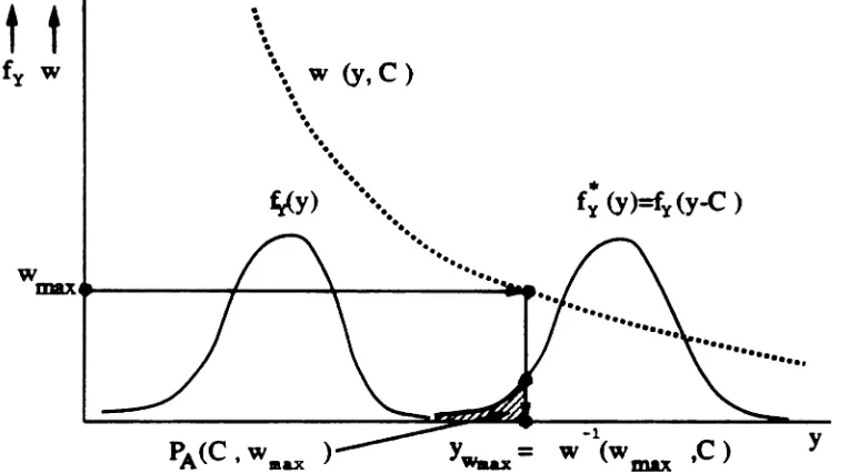
w(y,

C) represent the weight function

.,(" C ) =

/Y(J/)//;(r)

=

h(,)//Y(J/ - C)

and 17'" be the indictJtoror counting function (equal to 1 if and only if,.

>

T

and equal to 0 otherwise). Since w(,.,C)

>

0 and 0 ~ 17''' ~ 1,

1 N 1 N

- E

17'''-('',C)

< -

E

max

{_(,.,C)}

= mo:

{1II(',,0)}

(3.1)

N N L-_l

for any translation amount C. In order to prove the first part of the theorem above,

we only need to prove that there exists a C",in such that

for C

=

Crain.

Let 11

=

w-1_{(W, C) be the value ofY such that}

w(y,C)

=

/y(y)j fy(y -

C) = W

for some weight W. That is, w-1_{(lV,C) is the inverse weight function parameterized}

by the translation parameter C. Furthermore, when the translation parameter is equal to C, let PA(C, W) be the probability that a single decision will correspond to a weight greater than W, and Ps(C, W) be the probability that all N decisions will correspond to weights less than W. Since decisions are independent,

Then, assuming that w(y,C) is non-increasing with y, Cm in above ezUts and can be

found as the minimum C that satisfies the tail probability equation

Of, equivalently,

1

.-

1( .,. . . .,0)

- 0 0

Iv

(y - C) tly

=

1 -

'{jP

_{m in}

Clearly, when Gmin is chosen this way,

(3.2)

and max {W(rll'C"'in) }

::5

t o _ with probability equal to P"'i". Then,

with probabilityequal to Pm_and, thus, we have proved the tint part ofthe theorem. Figure 3.1 lives a schematic illultration of the above.

y

•

r,

(y)=fy(y-C )

-1

W (w

max

.

..

.

....

_{••• W (Y,C )}

.

•.

.

.

..

....

...

..

~y) - ,

..

...

...

PA(C t W )

.ax

W

max.---...---~----

..._

t t

fy W

Figure 3.1: Memoryless case: schematic illustration of underestimation proof, part 1

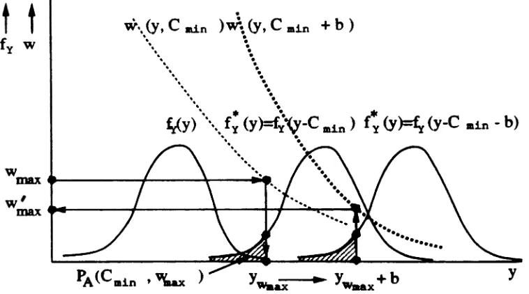
To prove the second part of the theorem let J/-.ae

=

w-1( Wmae ,Gm in ) and b be

any positive number. According to the first part, for G

=

Gm i n

+

b~ G",in, max {

tD('II,

CMin

+

II) }

<

w:.u.

= 10('...

+

6,C..m

+

6)

with probability equal to Pm i ft • Our only assumption about the pdCil that

Iy(r+

b)~

/y(,) [i.e., the pdf is Don-increasing in the tails), which i. Dot reltrictive for most

realiItic pdf'•. It follow. that

- fY(Jlw•••

+

b)/

h(J/",•••

+

b - Cmin - b)

fy('II"'....

+

b)//Y(JI - Cmin)

<

!Y(JI )//Y(JI - C"'in)

This implies that, for C ~ _Cmin and with probability P",in, the probability of error

willbe underestimated by an even larger amount than in (3.4). Figure 3.2illultrates the above.

t t

r,

W

.

.

.

.

"

...

.

~y) •••., fy (y)=fy~-Cmin) fy (yFfy (y-C min - b) ,

.

.

.

,

.

'.

.

".

.

..

'.

.

VV_{max ---I---~~-...}'. ~

..

..

VV' ~

max

Figure 3.2: Memoryless case: schematic illustration of underestimation proof, part 2

Note that equation(3.1) is always true for the maximum weipt occurring in each

simulation. That ia, theestimate

P

e is always bounded hom above by the maximum

value the weight function takes:

t:

$ max {

w<S,.,

C)}. In fad, Lu and Yao in [24]

have used similar arpmentl when they proposed analytically minimizinS a 60und

presented arguments is that over-translation causes the bound W_moe on the maximum

occurring weight to be smaller than the true Pe most of the time, therefore resulting in underestimation of Pee The slisht complication of the proof Items hom the fact

that Dot only the probability of a liqIe random weisht being greater than a preset

maximum Wmoe [i.e., the tail probability PA(C,tD"...)) mUlt below, bat &lao the probability PB(C,wmae ) of &ll weights being leiS than 10. . . must be lUsher than a given Pm in •

We have shown that over-translationwill resultin underestimation with high

prob-ability by showing that, under mild conditions, given an amount of underestimation and a probability (close to 1) that this underestimation should occur, one can find an

amount of translation that will underestimate at least as much, with a probability at

least as high. The arguments that were used constitute a rather conservative proof and therefore, the resulting bounds on parameter C are accordingly loose. In

prac-tice, underestimation will be observed consistently for smaller values ofC, as verified

by experiments.

As an example, consider the case where the noise pdf is Gaussian with mean zero

and (1'

==

1. Then, for a decision threshold T

=

5.6, the true Pe willbe P, ~ 10-8•

Assume translation by C. Let N

=

50,000. We set WmclZ =

10-10

and Pm in

==

1 - 10-8 • Solving [numerically] (3.3) for Cm in we find Cm in ~ 16. This means that,

for C

>

16 our estimate will be Ie•• tAanWmae = 10-10 with a probability ofat least

3.3

System with Memory: Direction of Biasing

We now focus our attention to the general multidimensional problem [i.e., when

memory and sipal are present and where the inputdiltributions are biased] which is

the one of practical importance. We as.ume that the "block" approach of (2.7) will be used. That is, we assume that the problem iI to obtain the optimal

c(j)

for each realization a(j), j = 0, ... ,J - 1 of A. The modified noise pdfwiD be

(3.5)

This implies that the IS estimator is given by (2.11). This approach has been used successfully in

[15]

for the case of additive Gaussian noise and has been shown to be superior to the conventional approach where no explicit conditioning on "realizations" is taken into account.

From a practical standpoint, the amount of effort required to obtain the J x AI IS parameters c(j,i), i

=

1, ... ,M implied by (3.5) seems unrealistically large -especially since analytical methods would not be helpful in the general case. Instead, letting the bias be along Borne directiond that remains fized for all realizations, that is, let ting c(j)

=

C(j) d for all

i,

reduces the degrees of freedom by a factor of M,

thus reducing the problem to that of finding J parameters C(j), one {or each real-ization. Clearly, unless the optimal biasing direction is known somehow in advance, there is a trade-off between parameter estimation effort and estimator efficiency. Our

experimental results indicate that by biasing in a lingle direction, large improvement factors are still achievable, provided that this direction that is chosen beforehand is

o

Figure 3.3: A 3-dimensional input noise space with an impulse response h, a biasing direction d and a decision surface S

It was shown in

[15]

and verified in

[16]

that, for a linear system with additive Gaussian noise, the optimal c(j) is copt(j)

=

C(j)h, where h is the impulse response

of the linear system. The idea of biasing along the direction of h seems intuitively appealing, even when the noise is not Gaussian. Since the optimal direction cannot be determined analytically, at least in general, we suggest using d

=

h as a reasonable heuristic choice when the system is linear.

Furthermore, the direction of h also seems to be optimal, for linear systems,

In a different sense: Let U be an orthogonal trtJu/ormaJion in RM, where U

=

[h, bJ, ... ,b..), and b,, i

=

2, ... ,M are column vectors in RM. Let D and D·

be the noise vectors before and after biasing. Let v and v· be random vectors such that D

=

U v and v· is the biased version of v. Then

n" - n

+

C(j)h

=

u

[v

+

C(;)[1,0, ... ,

O]T]

But 0* is also 0*

=

U V·. Therefore,

The biased output y. of the linear system will be

y. = hT n" = hTUv" = VI

+

C(j)

assuming

IIhll

=

1. This implies that, in the case of a linear system, translating in the direction of h has the potential of reducing the dimensionality of the problem to unity, with all the obvious benefits of reduced memory. Davis in

[13],

first suggested using an orthogonal Householder transformation to reduce the dimensionality to unity, and presented results based on the IS technique where the variance of the noise distribution is increased. This approach is also discussed in

[16]

for the Gaussian case in conjunction with the translation technique. Although it might not always be possible to actually implement the Householder transformation method for any noise distribution, this approach provides additional arguments in favor of the direction of

the impulse response, at least at the intuitive level.

As a last and most important argument in favor of biasing in the direction of

h, note that among all directions d, an additive bias C h mazimizfs the effect

0/

translation at the output of a linear .,.temsince, as shown in Figure 3.4,

y

-T

- h

x>

T

o

Figure 3.4: Linear system: a 2-dirnensional illustration of an impulse response h, a biasing direction d and a decision surface (hyperplane perpendicular to h)

of the input vector on the direction of the impulse response. The direction h can

thus be thought of as a mapping of the y-axis, with the decision threshold located T

units of distance from the origin (Figure 3.4). Therefore, biasing along this direction

clearly maximizes the effect of the translation, in the sense that out of all translations

with the same magnitude C

Ildl\,

translation in the direction

d

== h incurs the largest increase of error count.

For a nonlinear system, this suggests that a good biasing direction would be the

one in which the effects of translation are maximized at the output. In general,

the choice of good translation direction(s) for nonlinear systems willdepend on the

characteristics of the particular nonlinearity. We will present in the next section a

model for nonlinear systems that greatly facilitates the search for a favorable biasing

direction.

y == hT_{x and n" == n}

+

_{G(j)d. Then}

v'

hT n"

hT D

+

G

(j)

hTd

== hTn

+

GJJ

- y

+

GIJ

where Gil == C(j)hT_{d. Then (temporarily dropping the explicit reference to}

j)

(3.6)

and we conclude that for a linear system, translation of the joint input distribution by Cd always results in pure translation of the one-dimensional output distribution by Cy == C hTd. Now, if one wants to specify Gil at the output, say to achieve

a certain raw error count, there are infinite ways that this can be accomplished by

translating the input pdf's (the infinite solutions (G,d) to the equation Gil== GhTd). However, each one of these solutions would result in a different estimator variance (Eq. 2.14) and only one of them would correspond to the optimal biasing of the input distribution (i.e., to minimum estimator variance).

From a non-geometric point of view, and assuming

IIdll

== 1, the direction of bias can be thought of as the way of distributing the amount of output translation G_JJ over the input pdf's. It should be clear that, although the amount of translation Gil is important, the way this is distributed among the the input pdf's is crucial for the resulting estimator variance.

the unbiased case. Also, d such that dTh = 0 would imply C_w= 0, thul incurring no

difference on the output distribufion (y.

=

y). In fact, the whole half-Ipace defined by hTd

<

0 can be immediately rejected, since the l'eIulting tranllation at the output

is non-positive.

Clearly, d = h seems to be the most natural choice, although, to this point, no

general, rigoroua proof exists for itl optimality.

3.4

Nonlinear

SysteRls

Nonlinear systems are, in general, much more difficult to analyze from the IS

perspec-tive than linear systems. Although they are the very systems for which simulation is

most commonly needed, describing and modeling them,evenfor simulation purposes,

may be far from trivial. Attempting to apply IS techniques in a general and practical

way appears to be a formidable task.

At a first glance, one might suggest attacking the problem on a case-by-case basis, taking advantage of special conditions each time. However, such an approach

is not sufficient (clearly, simulation practitioners would not like having to approach

every nonlinearity as a totally new problem) and provides no further insight into the

problem.

A first step towards a solution for the problem is an attempt to approximate the nonlinear system with a linear Iy.tern. The authors in [14] proposed uling rqre,mn to estimate the coefficients of an efUivtJlent impu&e ruporue that approximated the

criginal eystem as close &8 poIlible. The obvious advantage of such a method it that, after a "linear equivalent" h.. been found, all the relultl hom linear IYlteDll can be

(13, 14, 25]). Unfortunately, and apart from being intuitively displeasing, the idea of

a linear approximation to a nonlinearity is meaningful and useful only for very mild

nonlinearities.

We Ingest ~oing a step further and using a more complex model, bycucading

a linear, time-invariant, causal IYltem to a memorrle•• nonlinear Iyltem. Fisure 3.5

shows such a discrete nonlinear Iystem.

Linear, Non-linear memoryII (instantaneous)

a

n

x

h

Wk

9 ( .)

Figure 3.5: Discrete nonlinear system model based on a cascade of a linear system with memory and an instantaneous nonlinearity

It follows that, at time sample n,

OD

'lin=

g(

Wn )

=

L

CI.,W'

'=0

and

OD

10" =

L

~Z,,-i

i=O

(3.7)

As shown in [3], pages 9-10,such a representation of a discrete nonlinear system is

equivalent to a tlucrete VolterrA serie» model. In seneral, the memory of the linear

part and the order of the nonlinear part can be infinite. In practice, however, we truncate the memory to M and the order (hicheet power) of the nonlinearity to K.

TlUs reeult. in a Volterraaeries representation with a finite numberofl1lIDDlatioDI of finite terms each. Note that such a model (Fipre 3.5) is very seneral and can describe

accurately any nonlinearity, usuming we allowM and K above to besufficiently larse.

It is also a compact, relatively simple model and is used extensively by researchers and simulation practitioners. Several techniques have been proposed to estimate the

coefficients of such a model, given a nonlinear system. In this work we will assume

that this system identification problem can be solved with acceptable accuracy.

Consider initially the case where the system consists of an instantaneous

(rnemo-ryless) nonlinearity: y(t)

=

g(z(t)) or Ylc

=

g(z.), for the discrete case. Then, '1/.

>

T is equivalent to g(z.)

>

T or ZIc E {lx, where Ox

=

{z :g(z)

>

T}. In general, an instantaneous nonlinearity is merely equivalent to a transformation (mapping) of the

one-dimensional output space important region to the one-dimensional input space.

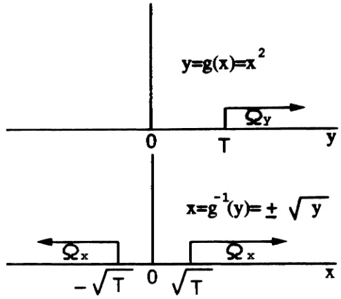
For example, if g(z)

=

Z2, Oy

=

{y : y

>

T} maps to

nx

=

{z : z

>

.jT

or z

<

-vT}

as Figure 3.6 shows.

Therefore, in the IS context, in order to increase the number of occurrences of

important events 'II E

ny,

we should somehow increase the probability of z E Ox that is described by the mapping 11

=

g(z) or, equivalently, z

=

,-1(,).

Assume now that a linear system with memoryM and impulse response h precedes

the instantaneous nonlinearity ,(.), as predicted by the general model wedescribed

earlier

(Eq.

3.7,3.8). Referrinr; again to Figure 3.5, to

=

hT

x

and 11

=

g(

to).

Then,to

2

y=g(X)=x

o

T

y

y

-IT

0

IT

x

x

Figure 3.6: An example of the mapping induced by an instantaneous nonlinearity

h becomes a mapping of the w-axis. The important region Oy (typically a threshold-type region, y

>

T) is mapped on one or more regions of the w-axis or, equivalently,

of the direction of h. For example, if !ly = {y : y

>

T} and y = g(

w)

= w3

then Ow = {w : w

>

{IT} and Ox = {x : hTx

>

{IT}. If y

=

g(w)

=

w2 _then

!lw

=

{w : w

>

VT

or w

<

-VT}

and !lx

=

{x : hTx

>

VT

or hTx

<

-VT}.

Figure 3.7 illustrates these examples for M = 2.

In most realistic cases nonlinear systems are operated in the range where g(.)

is monotonic. Assuming monotonicity, Oy

=

{y : y

>

T} and'll

=

g(w) imply

Ow = {w :w

>

g-l(T)} and Ox = {x : hTx

>

g-l(T)} (an increuins fuDctioD was

assumed, without lOIS of generality). In the IS context this implies that an approach

similar to that taken in the linear case can be used, where T will be substituted by

# #

I I

...

I

Qy •

T

(8 )

y

w

Xl

T

Y

w

Xl

( b)

Figure 3.7: A 2-dimensional illustration of the mapping of important regions for a nonlinear system

runtime savings, comparable to those achieved when the systemi. linear.

If g(.) cannot be assumed monotonic in the entire operating range the problem becomes more complicated. We can distinguish two interesting cues:

(i) Ow is of the type

Ow

=

{w :w

<

1'1

or w >

1'2}

Then, a split-and-translate scheme could be applied [25], where the pdf is Iplit in two identical parts (with probability leach) that are translated in the two opposite directions. Due to symmetry, and for all practical purposes, this scheme will have effects identical to simple translation and can be analyzed in the same way.

Figure 3.9: Input space and important regions when Ow

=

{w :w

<

1'1

or 10

>

1'2}

where

11'1 - 1'21

is assumed larse [i.e., many standard deviations of the pdf involved).

Then, the scheme proposed earlier can still be applied, U8Umin~that over-translation

will never cause the modified pdf to have sisnificant valuel beyond

1'1

(i.e., "Ipill-over"

beyond the important rqion).

~" _~~~~:

: /

,:" _.'- ""~'-' _W

,'~~~,,~,,-" _~~

~'-'"

~..

,.

.~~~~ .'~ ,..",

.,li

-

...,'-'

.~.,-f.,(w)

_{~ ~~'''~} \.

"~.~~~ ~~

".

.'-,-",-"-

""

~" ~~,

~_~s~~*~~~.,

,~"-.,.,~~~~~ ~''':.' _~ ,S~

h

~:\'~~" ""

."'-~~~

'" :...

'-~I\ :'\." ...

~:\ .,.. ~.

,..", ,,~,_.:.'\:'~"4: ... _,~~. _~,"" , " ' "

~"\.:'"-"

T2

'~~. ... ~,,:\~,~~:

...

o

Figure 3.10: Input space and important regions when Ow

=

{w :

1'1

>

W

>

1'2}

Figures 3.9 and 3.10 illustrate, respectively, cases (i) and (ii).

Ifg(.) is non-monotonic and does not fall in these two categories then, in general, biasing by translation may Dotbe advantageous and the problem should besolved on

3.5

System with Memory: Effects 01 Over- and

Undertrans-lation

AlBumins DOW that the modified pdf i. siYeD by (3.5), where

e(j)

=

aUld

and

.

d

=

(Ill' ...,dl l] has been chosen appropriately, weloc1ll our attention to the problem

of estimating near-optimal parameters C(j) for each realisation. ArsumeDt. Iimilar to those used {or the memorylesl cue can be used to jUltify the obeervatioD that,

when C(j) is too large, underestimation occurs with high probability.

Theorem 2. Let the true probability of error, under the H_o hypothesis and real-ization

i,

be Pe(j), and the ISestimator (when translation is used) be Pe(i). Assume

that the system under consideration can be represented by the equation y

=

g(o),

where n is an M-dimensional input vector. For any given WO t mtlE = a,Pe(i), where

o

<

a

<

1, any number of decisions N and any arbitrary Pm in , a translation amount

Cmin(j) exists such that, for C(j)

=

Cmin(j):

Furthermore, for any C(j) ~ Cm in ( ; ) , Pe(j) willbe underestimated by an even larger amount, i.e., Pe{j) ::; w~,mae ::; Wo,mae, with probability Pmin.

Proof: Let wo(y,C(j)) denote the output weisht function and wij(ft,

CU»)

the

weight function of the i-th input pdf, under realization j. Let Jill denote the i-th

decision sample in a simulation and "ki denote the i-th element of the corresponding

and equal to 0 otherwise). Since wo(y,C(j»

>

0 and 0 ~ Ir,. ~ 1,

(3.9)

{or any translation amount C(j). In order to prove the firlt part of the theorem, we

·only need to prove that there exists a Cmin(j) suell that

for C(j) == Cmin(j).

Let n == W;l(W, C(j)) he the value such that wi,;(n,C(j))

=

W for some weight

IV. That is, W;l(W,C(j)) is the inverse weight function (for the i-th input pdf) parameterized by the translation parameter C(j). Furthermore, when the translation parameter is equal to C(j), let PA(C(j),1'\-') he the probability that a lingle decision will correspond only to input weights greater than W, and PB(C(i),

»')

be the prob-ability that all N decisions willcorrespond only to input weights less than li'. Since decisions are independent,

P

s (

C(j),ll')

=

(1 - PA (C(j),W))N

The input weight functions are assumed to be non-increasing with n. Assuming mutual independence of the input samples, the total weight for each output sample is given by the product of the corresponding input weishtl (Eq. 2.12). A way to force output weipts to be less than Wo,mCle is to make input weights be less than

Wi",_ = ~100,_. Then, C_in(i) above eNU and can be found as the minimum

C(j) that latisfies the equation

or, equivalently,

M M w~

llpr

[WiJ(n,C(j» ~ Win,_]

=

lll(C(j), cia)

=

YP..

n

i=1 i=1

(3.11)

where C...,,(;)

>

0, I(O(j),

cia)

are int.a1a [i.e., tail probabilities) of the form

Clearly, when Cmin(j) is chosen in such a way,

Pm in ,

in which case, both

max {wi,;(nki,Cmin(j)) } ~ Win,mac

and

with willhold with probability equal to Pmin- Then,

(3.12)

with probability equal to Pm i n , which proves the first part of the theorem. Fip.re

3.11 illustrates schematically these facts along one of the input dimensions.

To prove the second part of the theorem let n.i...,i = Wi"J(Wi",,...,

C",.{j»

and b

(n-C(j)d. )

I

-1

Ilw = w (w

in , max i,j intIDlX ••••••••; 'i,j (Y,C

o»

.•.

••

..

••_••

••••_••

..

••

•••• f· t,8~

' . .1:) 1:1 ••••_••

••_••

••

~I j (n)

w. III,IDU

Figure 3.11: System with memory: schematic illustration of underestimation proof,

part 1

and

(W~n,ma~)M

both with probability equal to Pm in . Invoking the non restrictive assumption that

and, therefore

error willbe underestimated by an even larger amount than in

(3.12).

Figure 3.12

illustrates the above.

w1:;.(0,

.

Cain

e»\

.

Wi,j (0,CaiD (j)+b)

..•.

.

\

.

.... \.. f· (n\-I' (n-C (j)A -b( 1 )

...

•••• H'

j "-"1:J IUD ~

f:,

j

(i.>:j.1

j

(O-\:D

(j)d_{i )}

~'j (0) •••••• •••••

.

.

...

'<,

Figure 3.12: System with memory: schematic illustration of underestimation proof, part 2

As in the memoryless case, equation (3.9) is always true, that is, Pe(j) is less than the maximum output weight occurring in the simulation: Pe(j)

:5

max{Wo(Yk,C(j))}.

Our purpose was to show that this maximum weight will eventually become very small with high probability when the input distributions are over-translated, thus_, resulting in underestimation of Pe(i). Some added complexity stems from the lUsher dimensionality of this cue with respect to the memorylese cue. Equation

(3.11)

is

indicative of the fact that the probability of an input weight being pater than a preset maximum is now the product of M tail probabilities. Thefact that alloutput weights mUit be less than the prespecified bound 100 ,. . . i. taken into account by

As an illustrative example, consider the case where the input pdf's are

Gaus-sian with mean zero and tT

=

1. Let the system be linear with

M

=

3 and

h

=

[-0.5,2, -0.5]. The outputwill be Gaussian N(0,4.5) and for a threshold T = 12,

Pe ~ 10-'. Assume translation by e = Ch. Let N = 500. We set tD.._

=

10-10 and P",in

=

1 - 10-2• Then tDin,_

=

-VW..-

= 4.641

x

10-4 • 80lvins (3.11) for

em.i.n we find Cain ~ 20. This means that, for C

>

20our estimate will be

te••

UuJn

Wo,mae = 10-10 with a probability of at least P_{m in} = 1 - 10-2 •

As pointed out earlier, the bounds on C and C(j) implied by (3.3) and (3.1i) are very conservative, and are used here only in order to rigorously prove the high proba-bility of underestimation. In actual experiments, underestimation occurs consistently for values of C considerably less than those predicted above.

Turning our attention to the other extreme case of interest, when C is relatively small, we observe that the biased input pdf's f* are still very similar to the original pdf's

f

and their behavior resembles strongly that of the (unmodified)

Me

case. As-suming a low Pe and a very small number of decisions, N, no errors willbe generated

in most simulation runs and the corresponding estimates will be

P

e = 0, thus

patho-logically underestimating Pe • In the rare case that one or more errors occur, the Pe

will be over-estimated because of the small number ofdecisions used - consider, for example, the case where p~

=

10-s, N

=

1000 and one error is detected. IfC is close to zero the weight corresponding to this error willprobably be large, I&y 10 ~ 0.001. This will result in an over-estimation:

t.

=

i

>

10-8• However, sinee this will be an

isolated, rare event, the overall behavior of the estimator in this ran~e of

C'.

will be that of underestimation.

AI

the tranllation amount C is increased from zero, the variance in the eetimate

close to the true Pee Eventually, when the translation amount grOWl well beyond

the "optimal" range of C'I and reaches the over-translation region, the estimator will

consistently underestimate the probability of error.

Combining these theoretical observations, we conclude that if the number of

deci-sions is very small with respect to the true Pcexpected, a typical plot of the reeulting

estimates as a function ofC for 0$ C $ Cmae willlook like the one in Fipre 3.13.

c

C toolow ---~~I C good C too high ----..

Figure 3.13: Typical curve of

P

e vs. C, for 0 ~ C ~ Cmoz

3.6

Proposed method

The above theoretical observations suggest the following heurUtic scheme to locate

optimal or near-optimal settings {orC, for a given direction d. For each realization

a(j), j

=

0, 1, ...

,J -

1:

oC the BER is usumed to be always available; even if this i. not true, N could be

later modified, as we explain in the Collowing. The choiceoC N depends on the actual

Pe and the variance reduction that is expected to be obtained by IS.

- Run a aeries of simulations with lenph N, where /NIi(n) i. traulated by

C(j)d, that is

ni(j)

=

Ri(i)

+

C(j)~, i

=

1, ... ,M

{or every block of M samples. Plot the curve of estimates

P

_e as a function of C(j)

{or 0 ~ C(j) ~ Cma,z, where Cmae is chosen to result in significant underestimation of Pee

- If N is not too small, the curve will consist of three distinguishable regions

corresponding to "C too low", "C reasonable" and "C too high". Then, a

near-optimal C(j) can be picked from the range where the curve is at its flattest, as shown

in Figure 3.13.

The choice of N together with the actual improvement {or good C's determines

the shape of the curve in a predictable way: When N is too large, the flat region will

be relatively wide making the choice of a good C more difficult (actually, this wide

flat region implies that, for the N used, the estimator varianceis less sensitive to the choice ofCin this range). When N is too small and/or the variance reduction is small,

behavior similar to the case where C is too small will dominate for the whole range

of C'I; that is, most estimates will be zeros with occasional over-estimation spikes.

The curve in this cue will never rise to a flat region before underestimation starts

occurring, indicatins that the N chosen is too small to

pve

reasonable estimates,

even for

C'.

close to optimal. In other words, the variance reduction of the estimator,

small N used. Figure 3.14 .howl typical curves expected for various choicesof N .

r:

.

t

...

..

-

..

\

\\

_\

Figure 3.14: Typical curves for various choices of number of decisions N

To maximize computational efficiency, it is better to start experimenting with an

N that might be too small and later increase it, ifneeded. Since the number N for

each run will typically be much smaller than the number that will eventually be used

for an accurate estimate of Pe' the overhead involved in using this method to find

good O's will be low. A useful byproduct of this trial-and-error process is & rough

estimate of the variance reduction expected for good O's ( the ratio of the number of

decisions that would have been used for

Me

simulation over the number of decisions

N that is actually used).

An

alternate, more efficient scheme, in the sense that less let-up simulation runs

are required, could exploit the prior knowledge of the shape of the curve and 11Ie a

Ongoing research is attempting to answer the question of locating the optimal

C more accurately within the flat region, and the robustness of the improvement

factor around this optimal. Moreover, the relationship between the raw error count

[i.e., number of errors occurrins at the output) and the optimal

C

it etill under

investiption. Our experiments indicate that very lUKe improvement factore can be

obtained even when we choose a value ofCin this resion almost arbitrarily, althoush

the point where thecurve exhibits maximum flatness seems to be the best choice. On

this last subject note that, since consecutive estimates

P

e on such a curve ditrer only

sligh tly in translation amountC, they can be considered (approximately) &8estimates

at the same value of C. Therefore, it appears that the local flatness of the curve (i.e., region where dPe(C)/dC ~ 0) is a good indicator of reduced estimator variance.

Clearly, a second statistical indicator of the goodness of the estimate as a function of C, would be very useful. Such a statistic, together with the one we propose

and maybe a more efficient search procedure would allow near-optimal translation parameters to be found within the actual simulation itself and not by previously run, exploratory simulations. A natural candidate for secondary statistic appears to be the sample variance (or coefficient of variation) of the BER estimates. At this stage, the practicality and reliability of such a statistic as well as the sensitivity of the improvement factor to changes of C in the flat region are still under investigation.

3. 7

SUIDIDary

Since the effects of under-translation and over-translation are predictable in the way described for a very broad class of pdf's, we conclude that the heuristic scheme we

near-optimal values for the translation parametersC(i),without requiring intractable analytical derivations.

In order to justify the observed effects of under- and over-translation, the

argu-ments presented above are not restricted to the cue of a linear Iy.tem. Therefore,

once a good translation direction d has been ehosen [e.g., d

=

h for a linear system), similar obeervatioDs can be used to determine whether the Clmount of traulation C

&lons that direction is too larse or too small. For nonlinear systems, the problem of

identifying near-optimal translation directions appears to be less simple in general; however, these difficulties can be surpassed in many cases by using the nonlinear system model (i.e., cascade of linear system and memoryless nonlinearity) that we

4

Importance Sampling for Single-Sided

Distributions

4.1

Background

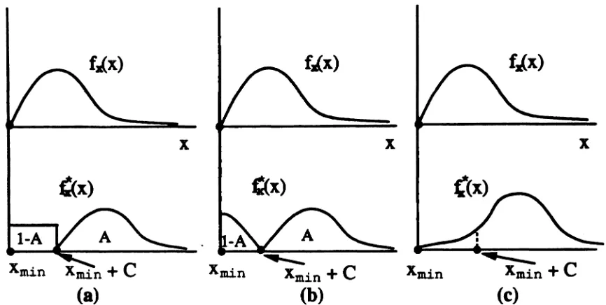
A class of noise distributions that has not attracted significant attention so far in the Importance Sampling context, is the class of single-6ided distributions. Let X be a random variable with pdf Ix{z). We say that X has a single-sided distribution when there exists an ZYnin such that

/ x (z)

=

0 ,for Z

<

Zmin

Suppose that we want to estimate the probability of the rare event {z EOx}, where

Ox is what we called earlier the important region. The fundamental rule when ap-plying IS techniques is that the modified pdf

Ii

(z) must be non-zero everywhere in Ox [10,12]. If

/i(z)

=

0 somewherein Ox, the varianceoftheIS estimator in (2.10) becomes infinite, resulting in underestimation of the true probability of an important

event.

When the important region is of the type Ox

=

{z : z

>

T} (the cue of binary detection with memory M =

1),

and li(z) = Ix(z - C), i~ is lufficient that C ~

memory, where the 'Yltem01ltput issiven by JI

=

g(x) and we are tryins to estimate

P,

=

Pr[,I

> T]

bymodifying the joint distribution of the input variables, fi(x) mUlt be non-zeroin Ox

=

{x Inch that II

=

g(x)

>

T}.

III thi. cue,it illeis obviouswhat

parts of the domain of X, D

x,

contribute to important eYeIltl, in other .orclI what

Ox is. Actually, for many Iyllema, linear or Donlinear, Oz can very

weD

cover the

tDhole domain Ds- It foBows that it is impOilible, in

ceneru,

to apply IS hued on

pure "linear .hift" or "translation" of the input pdf'., ifthese pdf'. are liJasIe-lided. A good example of a single-sided distribution with practical importance that was a strong motivation for this discussion, is the pdf describing the output current of

an Avalanche Photodiode Detector (APD) in lightwave communication systems. The widely used approximation obtained by Webb, McIntyre and Conradi in [26] (referred to in the following as the WMC pdf), is given by

(4.1)

for z

>

-Jii

p /Fe' where

X

is the mean output current, (T2 is the variance of the

current and his a shape parameter and

X

= (neq/at)G

q

=

charge ofan electron

t1t = time interval

G = average avalancheSain

fte = ("4t/lO)p. = number ofprimary electrons at the input oft.he APD " = quantum efficiency of the diode

Popt

=

averase optical power in time l1t

Ml

=

eaew of a photon

(T2 = ftc(/J

F.(q/ 4t)'

=

variance of the diode output current

6

=

v;&;T./{F. -

1)

Fe

=

Ita

+

[2 - (I/G)](1 - ') = excess noise factor

The properties of this pdf were studied in the context ofefficient simulation in (6]

and [27].

The Shot noise afFecting an APD i. a typical example of noise that is not i.i.d. and additive. In fact., the underlyiq noile pr