A statistical framework to combine multivariate spatial data and physical models for hurricane surface wind prediction
Kristen M. Foley1, Montserrat Fuentes1∗
1 Department of Statistics, North Carolina State University
Abstract
Storm surge is the onshore rush of seawater associated with hurricane force winds and can lead to loss of property and loss of life. Currently storm surge estimates are created by numer-ical ocean models that use a deterministic formula for surface wind fields. A new multivariate spatial statistical framework is developed to improve the estimation of these wind field inputs while accounting for potential bias in the observations. Using Bayesian inference methods we find that this spatial model improves estimation and prediction of surface winds and storm surge based on wind data for a case study of Hurricane Charley.
Key Words: Bayesian inference; non-separable multivariate models; spatial statistics; storm
surge forecasts; wind fields
*Correspondence to: M. Fuentes, Statistics Department, North Carolina State University (NCSU), Raleigh, NC 27695-8203, U.S.A.
E-mail: [email protected]
1
Introduction
Estimating the spatial and temporal variation of surface wind stress fields plays an important role
in modeling atmospheric and oceanic processes. This is particularly true for hurricane forecasting
where numerical ocean models are used to simulate the coastal ocean response to the high winds
and low pressure associated with hurricanes, such as the height of the storm surge and the degree
of coastal flooding. According to the National Oceanic and Atmospheric Administration’s (NOAA)
Hurricane Research Division more than eighty-five percent of storm surge is caused by winds pushing
the ocean surface ahead of the storm. The numerical ocean models used for storm surge forecasting
are also driven primarily by the surface wind forcings. Houston and Powell (1994) did an analysis
of the impact of wind field forcings on the storm surge forecasts used by the National Hurricane
Center (NHC). They concluded that up to 6 hours before landfall, real-time model runs can be
used to evaluate warnings and assess the extent of storm surge inundation. Houston et al. (1999)
state that “an accurate diagnosis of storm surge flooding, based on the actual track and wind fields
could be supplied to emergency management agencies, government officials, and utilities to help
with damage assessment and recovery efforts.” Our objective is to use all available sources of wind
data in order to improve the estimation of the wind field inputs. It is expected that improving these
inputs will have a great impact on real-time storm surge estimates, allowing recovery efforts to be
organized immediately after a hurricane has made landfall according to the areas most impacted
by the storm.
Several studies have investigated the potential of using real-time observation-based winds to
improve storm surge predictions as new wind observations have become available from the
Hur-ricane Research Division (HRD). Since 1993 the HRD has reported real-time analyses of tropical
cyclone surface wind observations for evaluation and eventually to be utilized by the NHC
(Hous-ton and Powell, 1994). Powell and Hous(Hous-ton (1996) did a study of Hurricane Andrew (1996), and
concluded that real-time wind fields would improve storm surge forecasts, particularly for storms
with asymmetric (i.e. non axis-symmetric) wind fields. Houston et al. (1999) used the HRD winds
as input into a two dimensional storm surge model. In their analysis they did not allow the wind
and surface pressure fields were steady state for over 24 hours.
We propose a new method to use the HRD data to fit a statistical model for the winds that can
be used as input into a numerical ocean model. The statistically-based winds are a function of the
hurricane’s location and can be updated at intervals as small as 10 minutes as more observations
become available. A statistical framework is used to account for systematic and random errors in
the observations while using these observations to model the surface winds as a multivariate spatial
process. This is the first time that these methods have been applied to an ocean model application
to be used for improved storm surge forecasting.
For coastal ocean modeling we use the Princeton Ocean Model (POM), which is adopted by
NOAA as the operational coastal ocean forecasting system for the U. S. East Coast. POM is a
fully three-dimensional numerical model and has the capability of modeling the evolution of ocean
processes at many layers. In addition, POM includes open boundary conditions to account for
surface wind stress and a bottom following sigma coordinate system to account for differences in
water depth. As a result, the POM model is able to predict storm surge with greater spatial
resolution and temporal accuracy than simpler models with very few layers or quasi-geostrophic
dynamics which often cannot capture the large topographical variability of the coastal regions.
Unlike global and other large scale forecasting models, this model can be applied at a higher
resolution to a much smaller regional domain. Using statistical methods to combine observed data
and model output at this smaller scale is very challenging but it will ultimately have the greatest
impact on the health and safety of citizens living along the coast.
The statistical modeling of spatial processes in the atmospheric sciences has been an active area
of research over the past decade. Hierarchical Bayesian methods have been found to be particularly
useful for such applications, e.g. see Wikle et al. (1998), Berliner et al. (1999) and Royle et al.
(1999). Such methods have been applied to modeling wind fields. Wikle et al. (2001) present a
hier-archical spatio-temporal model for surface wind fields over the tropical oceans. Fuentes et al. (2005)
propose a method for predicting coastal wind fields based on a non-stationary and non-separable
covariance model that accounts for bias in available observations. In both of these studies the
apply generalized autoregressive conditional heteroscedastic (GARCH) models to the bivariate wind
vector at a single spatial location. In our statistical framework we combine all sources of available
data including a physics-based wind model and the observational data currently available to NHC
for coastal ocean prediction along the Eastern coastline. We investigate the importance of
account-ing for the cross-covariance of hurricane surface wind fields. The ultimate goal in the application
presented here is to develop methods that would be practical (in terms of computing time) for a
real-time forecast or nowcast scenario. Hence the sophistication of any proposed methodology must
be constrained by the computing demands of the method. The scientific question of interest is how
to balance the sophistication of the wind field model with computational cost.
Section 2 describes the deterministic physical model for surface wind fields, the available
ob-served data and the proposed statistical model. Section 3 reviews statistical methodology for
multivariate data following the linear model of coregionalization used in this paper. We outline
a hierarchical Bayesian approach for estimation of parameters in a deterministic wind model and
prediction of gridded surface wind fields. Section 4 describes the results of a case study for wind
field data from Hurricane Charley in August of 2004. The estimated wind fields are used to
ini-tialize the numerical ocean model and are shown to improve storm surge prediction. A concluding
discussion is given in section 5.
2
Data and Scientific Problem
2.1 Modeling Surface Wind Fields
For coastal ocean modeling we use the Princeton Ocean Model (POM), which is a three-dimensional
primitive equations ocean model (Blumberg and Mellor, 1987). Surface wind fields are the most
important input variable used to initialize the numerical ocean model to simulate the coastal ocean
response to hurricanes. A wind field is made up of wind vectors defined at a finite set of grid points
such that each vector has a magnitude or wind speed value (typically measured in meters per second
or knots) and a direction. These vectors are decomposed into orthogonaluwinds, (East-West) and,
of wind data at different locations in order to predict the wind fields at the grid locations used
by the ocean model. Let Vt(s) = (ut(s), vt(s))T be the underlying unobserved spatial process for
the wind components at location s and time t. We use the standard Cartesian decomposition to
define the wind vectors since the observed and predicted winds provided by NOAA are based on
this decomposition. However we note that other decompositions are possible and in particular the
u andv components could also be defined according to the direction of the motion of the storm at
a given time.
Currently for storm surge forecasting a deterministic wind model is used, referred to as the
Holland wind model (Holland, 1980) which determines the wind velocity induced by the hurricane
pressure gradient under cyclostrophic balance. The Holland wind model for surface wind speed at
a given location s is:
W(s) =
" B
ρ
Rmax r
B
(Pn−Pc) exp−(Rmax/r)
B
#1/2
(1)
Pnis the ambient pressure,Pc is the hurricane central pressure,ρ is the air density (fixed at 1.2 kg
m−3
), and r is the distance from the hurricane center to locations.
Under the assumption that the hurricane wind field is axis-symmetric the u and vcomponents
can be determined from the wind speed:
uH(s) =W(s)sinφ (2)
vH(s) =W(s)cosφ (3)
where φ is the inflow angle at site s across circular isobars toward the storm center. That is, for
every location the covariates foruandvare the radius (r), and angle (φ). The wind components are
a nonlinear function of these covariates with parameters θH = (B, Rmax). The forcing parameter
Rmax is the radius of maximum sustained wind of the hurricane. In the Holland model the
maximum possible wind speed in the storm is a function of the central pressure of the storm and
the valueB which defines the shape of the pressure profile. Large values of B correspond to a wind
will mean high wind speeds across a greater radius of the storm. These parameters are typically
based on results from previous studies and are held constant for all forecasting time periods.
Although this physical model incorporates important information provided by the observed
central pressure and the location of the eye of the storm there are known deficiencies in this
formulation. For example, the Holland winds are symmetric around the storm center, however
it is known that wind speeds are typically higher on the right hand side of the hurricane (with
respect to the storm movement). Various adaptations of this physical model have been proposed.
Xie et al. (2006) create an asymmetric model by incorporating data provided by the National
Hurricane Center (NHC) guidance on the maximum radial extent of winds of a given threshold in
the four quadrants of the storm. The NHC uses a parametric wind formula similar to the Holland
model to force the ocean model. Another approach would be to use a coupled atmospheric-oceanic
numerical model to simulate the surface winds at the boundary layer of the ocean model. Global
mesoscale numerical weather forecasting models such as the Mesoscale Model (MM5) and the
Weather Research and Forecasting Model (WRF) are capable of making forecasts for surface level
wind fields. However these forecasts are not suitable for real-time forecasts of hurricane winds.
Historically these models have been unable to accurately reproduce the intensity of hurricane force
winds. More recent reports show that MM5 and WRF are able to obtain more realistic wind speeds
when run at high resolution (on the order of 1 km grid size). However the CPU time required to
produce these modeled winds prevents such model runs from being used in real-time applications.
The best approach for regional storm surge forecasting is still using parametric hurricane models,
as discussed in Xie et al. (2006). For further details on storm surge forecasting for the coastal ocean
and estuarine systems see Xie et al. (2004), Peng et al. (2004), and references therein.
Here we focus on the operational methods and observational data currently available to the
NHC for coastal ocean prediction along the Eastern coastline and incorporate this information into
a statistical framework. In our analysis we provide a new tool to estimate the parameters of the
Holland wind function. We include the Holland winds as the mean function of a spatial statistical
model and incorporate a spatial covariance to account for any structures in observed hurricane
surface winds not captured by the parametric wind fields. This approach to wind field modeling
prediction.
2.2 Wind Data
There are three sets of available wind data to be used in hurricane forecasting and hindcasting. Data
provided by the National Hurricane Center (NHC) specifies the location of the storm center and the
central pressure. The NHC provides forecasts every 6 hours on the location of the hurricane center
(in degrees latitude/longitude) and sustained wind speeds (nautical miles) in different quadrants
of the storm. For historical datasets such as these there is also “best” track information for the
hurricane center and central pressure based on all available observations along the coast. The track
information is necessary when creating wind fields based on the Holland wind model. We use linear
interpolation to interpolate the best track information to estimate the storm center and central
pressure at ten-minute time intervals.
In addition, data on wind speed and direction at over 20 buoy locations along the Eastern
coast is available from NOAA’s National Data Buoy Center (NDBC). For this study we use the ten
minute average wind speed (m/s) adjusted to a common height of 10 meters above sea level and
ten minute average wind direction. Ten minute averaging times are considered to be representative
of the timescales typically associated with oceanic response to surface stress (Houston et al., 1999).
The wind speed and direction are then converted to uand v components.
Finally, gridded wind field data is available from NOAA’s Hurricane Research Division (HRD).
These wind fields are a combination of surface weather observations from ships, buoys, coastal
platforms, surface aviation reports, reconnaissance aircraft data, and geostationary satellites which
have been processed to conform to a common framework for height (10 m), exposure (marine or
open terrain over land) and averaging period (maximum sustained 1 minute wind speed). The
processing and quality control of the data use accepted methods from micrometeorology and wind
engineering and provide the best available near real-time gridded hurricane wind analyses. However
it is important to note that validation studies have shown that the HRD wind analyses are highly
variable in accuracy, depending on the quality and quantity of the observations used, and on the
(1999) report the gridded wind fields have been found to have estimated errors of up to 10%-20%.
For this reason although buoy observations are used to create the HRD wind fields we use observed
winds from the NDBC buoy network as a second data source to provide an estimate of the bias in
the HRD analysis fields. For more information on the HRD data see Powell et al. (1996) and Powell
and Houston (1996). HRD data is typically available at 3 hour intervals. HRD gridded fields are
provided at a resolution of approximately 6km×6km with the number of grid points on the order
of 104.
2.3 Statistical Model for Data
We use a statistical framework to account for the difference in uncertainty associated with buoy
and HRD analysis data. As described in the previous section the observed winds at the buoys
are considered more reliable compared to the HRD analysis data which has been shown to have
potentially large biases. This does not mean that no bias exists in the buoy data. For example
wave distortion effects have been found to result in a negative bias when deriving wind stress from
low-level anemonometers (Large et al., 1995). All of the buoy observations used in this study have
anemometer heights that are at least five meters above mean sea level. In fact more than half of
the sites are at heights greater than ten meters and so should not be influenced by surface waves.
We cannot hope to accurately estimate the bias of both data sources but only the bias of the HRD
data with respect to the buoy data. We take this approach since past studies suggest that the
maginitude of the bias in the HRD data, which includes satellite and ship data, is larger than the
potential bias in the buoys.
LetVat(s) = (va
t(s), uat(s))T be theuandvcomponents provided by the HRD analysis at timet
and locations. Let Vbt(s) = (vbt(s), ubt(s))T be wind data from the buoys timetand locations. For
now we consider time fixed and suppress the time index. We model the observed data as a function
of the underlying true (unobserved) wind process V(s) = (u(s), v(s))T. Then we model V(s) as
a multivariate spatial process with a mean function equal to the nonlinear parametric Holland
Measurement error (σ2
ub σ
2
vb)
Bias parameters
(au av)
Measurement error (σ2
ua σ
2
va)
Buoy Data Vb(s)
HRD Analysis Fields Va(s)
True Values V(s)
Physical Parameterization VH(s)
(Holland Model)
Stochastic Component ˜
V(s)
(Linear Model of Coreg.)
? ? ? @ @ @ I @ @ @ I
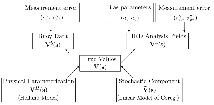
Figure 1: Model framework for wind components.
and b(s), as well as measurement error terms, ǫb(s) and ǫa(s):
ˆ
Vb(s) =V(s) +ǫb(s) (4)
ˆ
Va(s) =a(s) +b(s)V(s) +ǫa(s) (5)
Here a(s) = (au(s), av(s))T and b(s) = diag(bu(s), bv(s)) are spatial-temporal functions for
additive and multiplicative bias. These may be modeled as polynomial functions of location, spline
functions or as a function of additional covariates such as temperature or pressure. Based on
exploratory analysis comparing the buoy and HRD data we find that a multiplicative bias term in
not necessary and set bu(s),bv(s) = 1 for all locations s. Due to the limited number of buoy data
we consider only constant bias termsa(s) = (au, av)T for all locationss.
We assume both measurement error processes, ǫb and ǫa, are Gaussian white noise processes
with ǫb(s) ∼ N(0,Σb), and ǫa(s) ∼N(0,Σa) where Σb = diag(σ2ub, σv2b) and Σa =diag(σu2a, σv2a).
It is also assumed that these processes are independent of one another and the underlying process
V(s). It is possible to instead model the measurement error as a spatially correlated process with
some parametric spatial covariance function. We assume that the more complex spatial correlation
structure is captured in the model for the underlying true process and hence there is no need for
The statistical model for the unobserved “true” wind fields combines physical information from
the parametric Holland formula with a multivariate spatial process. The Holland equations (1) - (3)
define axis-symmetric wind fields,VH = (uH, vH)T, under cyclostrophic balance and represent the
large scale or mean structure of the surface winds. A multivariate spatial process, V˜ = (˜u,v˜)T, is
used to model the variability of the observed data that cannot be captured by any parameterization
of the Holland formula. We define the overall model for the underlying wind vector as:
V(s) =VH(s) + ˜V(s) (6)
We can obtain more reliable wind fields either by (1) introducing a more sophisticated
de-terministic wind model for VH (e.g. Xie et al. (2006)) (2) developing a sophisticated statistical
multivariate spatial model for the stochastic component ˜V. The proposed approach needs to be run
in real-time so a balance between (1) and (2) is the ultimate solution to the forecasting problem.
Alternatively, one could write a stochastic version of the deterministic model and approximate
the physical model using a stochastic spatial basis. This is the approach of Wikle et al. (2001)
for oceanic surface winds. Since the operational storm surge model uses parametric wind fields
(essentially like the Holland winds), it is preferable to instead provide tools to better estimate
the parameters of the Holland model accounting for uncertainty in the parameter estimates. This
motivates the problem of defining a multivariate spatial model for the stochastic component. We
adopt this approach here and evaluate the improvement in the wind prediction and storm surge
forecast.
3
Modeling Multivariate Data
3.1 Linear Model of Coregionalization (LMC)
In our setting, we account for any cross-dependency in the u and v winds by using a multivariate
spatial model based on a linear model of coregionalization. This approach was first introduced as a
of k unobservable factors withk < p. More recently, Schmidt and Gelfand (2003), Banerjee et al.
(2004), and Gelfand et al. (2004) proposed using this approach to construct valid cross-covariance
functions by modeling a set of dependent spatial processes as a linear combination of independent
spatial processes. We briefly describe the LMC model followed by a description of the steps for
Bayesian inference and prediction based on the available multivariate wind data.
We assume we are working with multivariate Gaussian processes. We find this is a reasonable
assumption based on analysis of the observed u and v velocities after subtracting off the Holland
mean function. In general, consider modeling p spatial processes V(s)˜ (p×1) for s ∈ D ⊂ R2. For
a finite set of locations s1, . . . ,sn, let V˜ denote a np×1 vector of the the p spatial functions
evaluated at these n sites: {V˜ : ˜V1(s1), . . . ,V˜1(sn), . . . ,V˜p(s1), . . . ,V˜p(sn)}. ˜Vj(si) denotes the jth
spatial process of interest at location swith j =1, . . . ,p and i =1, . . . ,n.
Letwj(s) beplatent independent Gaussian spatial processes with mean zero. Each process has
covariance function Cov(wj(si), wj(si′)) = ρj(si,si′;φj) with parameters φj, j =1, . . . ,p. These
covariance functions need not be stationary or isotropic. Now for w(s) = (w1(s), . . . , wp(s))T the
stochastic component in (6) is modeled as:
˜
V(s) =Aw(s) (7)
whereAis ap×pweight matrix that determines the covariance between thepvariables. Without
loss of generality we assume A is a full rank lower triangular matrix. This implies E(V(s)) =˜ 0
and
Cov(V(s˜ i),V(s˜ i′)) =
p
X
j=1
ρj(si,si′;φj)Tj (8)
where Tj = ajajT and aj is the jth column of A. Thus the cross-covariance is non-stationary,
depending on the form of the ρj. Also the cross-covariance function is non-separable, meaning we
cannot separate the between site variability and the variability between measures taken at the same
site.
Cov(V˜,V) =˜
p
X
j=1
Tj⊗Rj (9)
product. (Note, for V˜ = ( ˜V(s1),V˜(s2), . . . ,V˜(sn))T then the covariance is simply, Cov(V˜,V) =˜
Pp
j=1Rj⊗Tj.) Forρj stationary correlation functions,
Pp
j=1Tj =Tis the covariance matrix for
˜
V(s) so there is a one-to-one relation between matrix Aand matrixT. For p= 2,
T=
A211 A11A21
A11A21 A221+A222
(10)
Gelfand et al. (2004) also propose a non-stationary version of the LMC model by allowing
the weight matrix to be a spatial function, A(s). Since there is a one-to-one correspondence
between A(s) and the covariance matrix T(s), they develop an Spatial Wishart distribution for
T(s). However this leads to a nonstandard distribution for ˜V, e.g. the expression in (9) for the
cross-covariance is no longer valid since the weight matrix is now a random spatial process. We
thus propose to model all of the spatial structure within the latent processes. This will yield a
non-stationary model forV(s) whose properties are easier to derive and interpret.
Note that a separable covariance model is just a special case of the LMC model where ρj =ρj′
for all j, j′
= 1, . . . , p and ρj a stationary correlation function. In this case, Cov(V˜,V) =˜ T⊗R
for (R)ii′ = ρ(si,si′;φ). This is referred to as an intrinsic multivariate correlation model because
the correlation structure of the set of variables is independent of the spatial correlation. That is,
the correlation between two variables does not depend on spatial scale (Wackernagel, 1998):
Corr( ˜Vj(si),V˜j′(si′)) =
Tjj′ρ(si,si′;φ)
p
Tjjρ(si,si′;φ)Tj′j′ρ(si,si′;φ)
= pTjj′ TjjTj′j′
(11)
In the following application we apply both a separable and non-separable LMC model to the surface
wind fields.
3.2 Statistical Methodology
We now turn to the issue of estimation and prediction of the wind fields to be used in the ocean
for the parameters Θ = (θD, θH,θ˜) where θD=(a
u, av, σ2b, σa2) are the bias and measurement
error parameters, θH = (B, Rmax) are the parameters of the Holland model and ˜θ = (A,{φ j})
are the parameters for the LMC model for j = 1,2. We present a Bayesian framework that
allows for estimation of the parameters of the multivariate spatial model and the physically based
parameterized wind function while accounting for potential additive bias in the observed data. Let
ˆ
Vt= (Vˆbt,Vˆat) be all the available wind data at timetfrom the buoys and HRD analysis wind fields.
The posterior predictive distribution for the wind vector (u(s0), v(s0))T at a particular locations0
at timet is:
P(V(s0)|V)ˆ ∝
Z
P(V(s0)|Vˆ,Θ)×P(Θ|V)ˆ dΘ (12)
The full posterior predictive distribution (12) conditioned on the data from the na locations of
the analysis wind fields and the nb buoy sites can be approximated by using Markov Chain Monte
Carlo. We use a Blocking Gibbs Sampling algorithm (within the software WinBUGS, Spiegelhalter
et al. (1996)) to sample from the posterior distribution of the parameters by alternating between
the parameters of the underlying process, (θH,θ˜), and the parameters for the measurement error
and bias,θD. Our Gibbs algorithm proceeds in the following stages.
Stage 1:
Conditioned on the true wind processVwe obtain the posterior distribution of the parameters,θD,
that explain the bias and uncertainty about the data. The posterior distribution will be completely
specified once we define the priors forθD since we have:
P(Vˆb|V, σ2
b)∼N(V,Σb)
P(Vˆa|V, au, av, σa2)∼N((au, av)T +V,Σa)
Stage 2:
At the second stage we use the statistical model for the underlying true winds. LetVH denote the
output from the Holland model with parameters θH at the locations of the observed data. Thus
based on the conditional distribution:
P(V|θH,θ,˜ VH)∼N(VH,P2
j=1Tj⊗Rj)
and priors for (θH, ˜θ), we obtain the posterior distribution for the parameters in the Holland model
Stage 3:
We simulate values of V, the unobserved true process, at the na locations of the analysis wind
fields and the nb buoy sites conditioned on values of Θ updated in the previous two stages. Let
N =nb+na. The conditional multivariate distribution of Vat a new location s0 is:
P(V(so)|Vˆ,Θ)∼N(VH(so) +τTΣ−1[ ˆV−µˆ],Tˆ−τTΣ−1τ) (13)
where τ = ˆCov(V(so),V) is a (2ˆ N ×2) matrix and Σ(2N×2N) = ˆCov( ˆV,V). ˆˆ µ= (VH,a+VH)T
is the Holland mean function evaluated at the buoy and HRD locations accounting for the bias
in the HRD dataset. For more details on combining different sources of spatial data for Bayesian
prediction see Fuentes and Raftery (2005).
Thus after iterating through the three stages we haveMsamples from the posterior distributions
for the parameters,{Θ(m)},m= 1, . . . , M. The Rao-Blackwellized estimator (Gelfand and Smith, 1990) for (12) is
P(V(so)|V) =ˆ
1 M
M
X
m=1
P(V(so)|Vˆ,Θ(m)) (14)
Prior Specification
Uniform priors are used for the random effects such thatσb ∼U nif orm(.01,1) and
σa ∼ U nif orm(.01,5). We use relatively informative priors for the buoy data here based on
previous experience and analysis of similar datasets. These hyperprior values are based on
in-formation reported by the NDBC on the accuracy of the buoy equipment. The bias parameters
are assigned normal priors with au, av ∼ N(0, .001) (.001 is the precision). Priors for the
pro-cess parameters, θH = (B, Rmax), are chosen based on previous studies. B ∼ Uniform(1,2.5),
Rmax∼Uniform(15,55) based on the physical constraints described earlier and discussed in
Hol-land (1980). In the next section we describe the spatial covariance used for the hurricane case
study. For our application, φ1,φ2 are range parameters which we assign noninformative uniform
priors,U nif orm(10,1000), based on the size of the domain (in km) for the data.
Finally we must specify a prior for the weight matrix A. We take advantage of a conditional
computational cost of working with the fullnp×npcross-covariance matrix of the stochastic
com-ponent, Cov(V˜,V) =˜ Pp
j=1Tj ⊗Rj, in Stage 2 of the algorithm. Evaluating (9) for p = 2, the
joint covariance for the underlying true process V can be written as:
Cov(V,V) =
A211R1 A11A21R1
A11A21R1 A212 R1+A222R2
(15)
Now following a standard multivariate normal result:
u∼N(uH, A211R1) (16)
v|u∼N(vH +A21 A11
(u−uH), A222R2) (17)
Using (10) we can rewrite (16)-(17) in terms of the elements of the T matrix. Under the
new conditional parameterization we assign the scale parameters A2
11 =T11 and A222 =T22−T 2 12
T11
inverse gamma distributions (A12 11
, A12 22 ∼
Gamma(.01, .01)) and the weight parameter A21
A11 =
T12
T11 ∼
N(0, .001) (.001 is the precision). A similar approach can be used for multivariate data withp >2.
See the Schmidt and Gelfand (2003) study of multivariate air pollutant data for the conditional
and unconditional models for p= 3.
4
Analysis of Data from Hurricane Charley
In this section we apply the multivariate statistical model for hurricane surface winds to a case
study of Hurricane Charley of 2004. This case study was chosen because the hurricane surface winds
induced measurable storm surge along the coast of Georgia and the Carolinas. We compare four
different statistical models through a series of model diagnostics and look at posterior parameter
estimates for the separable LMC model for 6 time periods. An empirical Bayesian estimation
procedure is used for creating the gridded wind field inputs for the ocean model. Finally we run
the numerical ocean model using the estimated wind fields and compare the results to the predicted
Hurricane Charley crossed over the central Florida peninsula and moved offshore early on the
morning August 14th, 2004. Charley made landfall at Cape Romain, SC at 1400 UTC (Coordinated
Universal Time) on the 14th as a weakening Category 1 storm with highest winds around 80 miles
per hour (70 kt/hr). It then moved off shore again only to make landfall a few hours later at North
Myrtle Beach, SC. Water level gauges along the coast of Georgia and the Carolinas reported storm
surge heights up to 1.5 meters above normal tidal levels. We use gridded wind field data from
the Hurricane Research Division for 6 times on August 14th (0200, 430, 730, 1030, 1330, and 1630
UTC) leading up to Hurricane Charley’s landfall in South Carolina. For computational reasons we
sub-sample the gridded HRD data to reduce the number of grid points to the order of 102. Buoy observations from 23 locations are also used at these time periods to estimate potential bias in the
HRD data.
4.1 Model Estimation for HRD and Buoy Data
Our objective is to fit a joint model for the wind field vectors and obtain the posterior predictive
distribution of the winds at the ocean model grid points. Using the software GeoBugs (Spiegelhalter
et al., 1996), we fit four different models using 225 locations of the HRD gridded data for u andv
and data from the 23 buoys. Model 1 uses only the Holland mean function, i.e. ˜V(s) is neglected.
Note that in this case the parameters of the Holland winds are estimated using our framework
rather than fixed values based on “expert knowledge”. Model 2 treats the u and v components
as independent so that T12 = A11A21 = 0 in equation 15. Model 3 is a separable LMC model
outlined in section 3.1 so that the parameters of the underlying spatial processes are assumed to
be equal (i.e. φ1 =φ2). Finally, Model 4 is a non-separable LMC model which does not impose
this assumption about the spatial processes.
For this application, we assumeρj(si−si′;φj) are stationary correlation functions with
param-eters φj;j = 1,2. We did allow for geometric anisotropy, e.g. Fuentes et al. (2005), but found no
significant evidence of a lack of isotropy in the u and v winds for this case. Here we use an
expo-nential correlation function such that ρj(h;φj) = exp(−h/φj), j = 1,2 forh =||si−si′|| and the
uncorrelated.
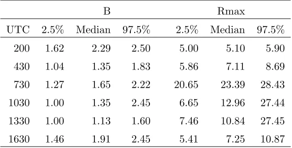
Table 1: Posterior medians and 2.5 and 97.5 percentiles for the Holland mean function in the separable LMC spatial model foru and v.
B Rmax
UTC 2.5% Median 97.5% 2.5% Median 97.5%
200 1.62 2.29 2.50 5.00 5.10 5.90
430 1.04 1.35 1.83 5.86 7.11 8.69
730 1.27 1.65 2.22 20.65 23.39 28.43
1030 1.00 1.35 2.45 6.65 12.96 27.44
1330 1.00 1.13 1.60 7.46 10.84 27.45
1630 1.46 1.91 2.45 5.41 7.25 10.87
Table 1 shows the posterior distribution summaries of the Holland parameters in the separable
LMC model for u and v. The parameter estimates are significantly different for different time
periods. Standard values for the Holland model areB=1.9 andRmax=35 to 55 km depending on
the size and intensity of the storm, e.g. see Hsu and Yan (1998). This range of values for Rmax
based on previous studies does not capture any of the values estimated in this case study. At 200 and
430 UTC the hurricane has just passed over Florida and is less symmetric. The radius of maximum
winds (Rmax) at these times is 5 to 7 km. Using the standard values greatly overestimates the
strength and extent of the winds at such times when the storm is less organized. We also note that
the cross-correlation values (T12/√T11T22) range from .24 to -.23 across the six time periods. The
posterior intervals for the correlation do not contain zero, suggesting there is significant correlation
between theu and v winds at all time periods.
Model Diagnostics and Calibration
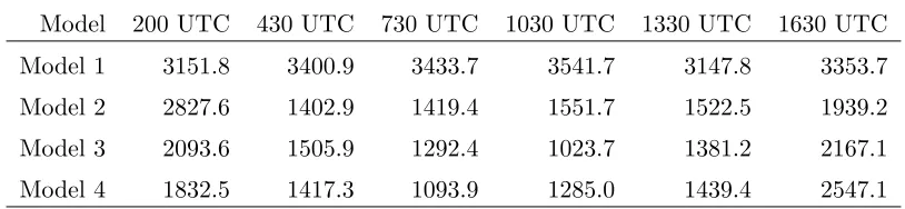
The Deviance Information Criterion (DIC) (Spiegelhalter et al., 2002) shown in Table 2 is used
to evaluate the different statistical models (where lower DIC values are better). All of the spatial
models perform much better than the model with just the Holland mean function. The multivariate
values for the independent and nonseparable models are similar. At 1630 UTC the independent
model appears to be the better fit. At 430 and 1630 UTC the eye of the hurricane is directly off
the coast and the wind speed contours appear more symmetric than the other time periods. Thus
although it is clear that the spatial models do a much better job of estimating the wind fields it
appears that the issue of independence of theuandvvelocity components depends on the structure
and organization of the storm at a given time.
Table 2: Deviance Information Criterion (DIC) Values
Model 200 UTC 430 UTC 730 UTC 1030 UTC 1330 UTC 1630 UTC
Model 1 3151.8 3400.9 3433.7 3541.7 3147.8 3353.7
Model 2 2827.6 1402.9 1419.4 1551.7 1522.5 1939.2
Model 3 2093.6 1505.9 1292.4 1023.7 1381.2 2167.1
Model 4 1832.5 1417.3 1093.9 1285.0 1439.4 2547.1
We use cross validation to evaluate how well the models predict winds at a new location.
Models 1 through 4 are used to predict at thirty HRD grid points that were not used for parameter
estimation. The median values of the posterior predictive distributions are used to compare to
the observed values at the hold out sites. Analysis of the cross-validation errors under each model
shows no significant prediction bias for any of the models. The non-spatial model using only the
Holland mean function has much larger error variance and several outlier values show that the winds
at a few locations are underpredicted by up to 15 to 20 m/s. The root means square prediction
error (RMSPE) values for Models 2, 3 and 4 (the spatial models) are very similar. We compare the
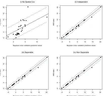
calibration for each model and each time period based on the 95% posterior predictive intervals. For
the models to be well calibrated the observed velocities should fall within the posterior predictive
intervals at least 95% of the time. Figure 2 shows calibration plots for thevcomponent for the hold
out sites at 430UTC. The prediction results for Models 2, 3 and 4 are practically identical. Similar
results were found for the other time periods and for theu winds. All of the spatial models have
calibration percents greater than or equal to 95% at all times. However the calibration percents for
Model 1 (the non-spatial model) are lower, ranging from 86.7% to 96.7%. Thus although the DIC
2, 3 and 4 perform well in terms of prediction. In fact it is not surprising that although the three
spatial models result in different covariance parameter estimates this does not have a dramatic
impact on spatial prediction (Stein, 1999).
4.2 Ocean Model Application
We now consider the application of the proposed wind field model for storm surge prediction. For
coastal ocean modeling we use the Princeton Ocean Model (POM), which is a three-dimensional
primitive equations ocean model that uses a finite differencing technique to solve the governing
equations and boundary equations. It has been designed to represent ocean phenomena of 1-100km
length and tidal-monthly time scales (Blumberg and Mellor, 1987). POM has been used in various
applications to model estuaries and bayes, semienclosed seas and coastal regions around the world
and has been applied extensively for studies in the Gulf Stream region (see Ezer and Mellor (1997)
and references therein).
In the previous section we used the fully Bayesian solution for the posterior predictive
distri-bution P(V(so)|Vˆ,Θ) outlined in section 3.2 to predict at 30 cross validation sites for six different
time periods. However, for the storm surge application we must create predicted wind fields for
every grid point of the ocean model domain for 96 ten-minute time increments over a period from
200 UTC to 1750 UTC on August 14, 2004. For this application the ocean model is typically run
at a resolution of 2 to 4 km grids. In our case the model was run using a resolution of 2 minute
longitude by 2 minute latitude grid (≈3.1km by 3.7km) with a total of 151×115 grid points. Hence
it is computationally infeasible to use the fully Bayesian prediction to predict the winds at a such
a high resolution.
Here we take an empirical Bayesian approach and use the posterior median values of the
pa-rameters, Θ, as the fixed “true” parameter values. Then the predictions are made following the
conditional distribution in equation (13). We compare the two methods based on the 30 cross
validation sites used in the previous section. Results show that the coverage is almost identical
for both the fully Bayes and empirical Bayes prediction. Also, on average, the widths of the fully
Figure 2: Cross Validation 430 UTC: Calibration plots for the vwinds at 30 cross validation locations for 4 models: (i) Model 1 – Holland mean with no spatial covariance (ii) Model 2 – independent (iii) Model 3 – separable LMC (iv) Model 4 – non-separable LMC.
0 5 10
−5
0
5
10
15
20
(i) No Spatial Cov
Bayesian cross−validation predictive values
HRD sites
−5 0 5 10 15 20
−5
0
5
10
15
20
(ii) Independent
Bayesian cross−validation predictive values
HRD sites
−5 0 5 10 15 20
−5
0
5
10
15
20
(iii) Separable
Bayesian cross−validation predictive values
HRD sites
−5 0 5 10 15 20
−5
0
5
10
15
20
(iv) Non Separable
Bayesian cross−validation predictive values
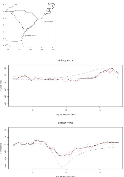
Figure 3: Map of 4 NBDC buoys within the POM domain. The remaining plots show the observed vwinds in m/s at each buoy in solid black for Aug. 14th 200-1750 UTC. The dashed and dotted line is the Holland output based on fixed parameter values (B = 1.9, Rmax = 46). The dashed lines are the predicted values and the dotted lines are 95% posterior predictive intervals using Model 3.
−84 −82 −80 −78 −76
30
31
32
33
34
35
36
(ii) Buoy 41008
(i) Buoy 41013
(i) Buoy 41013
Aug. 14 2004, UTC Hour
v−winds (m/s)
5 10 15
−30
−20
−10
0
10
20
(ii) Buoy 41008
Aug. 14 2004, UTC Hour
v−winds (m/s)
5 10 15
−30
−20
−10
0
10
Thus it appears that in this case the empirical Bayes prediction is a reasonable approach as well
as being significantly more computationally efficient.
We use the separable LMC model for prediction although, as noted earlier, the other spatial
models had almost identical results in terms of prediction. At the 10 minute intervals when buoy
observations are available but not the HRD datasets we use the parameter values based on the
estimation results from the last available HRD time when doing the prediction. For example, at
time 510 UTC the median values of the posterior predictive distribution forΘfrom time 430 UTC
would be used. In this way we have estimates at 96 different time periods corresponding to 10 minute
intervals between 200 to 1750 UTC on August 14th. Figure 3 shows the observed and predicted
v velocities for two buoys located within the ocean model domain. (Similar results were found for
the u component.) The dashed and dotted line is the output from the Holland model using fixed
parameter values (B = 1.9,Rmax= 46). The Holland function is unrealistically smooth and tends
to exaggerate the change in the winds as the hurricane approaches these locations. There is also
no measure of uncertainty in the values from the Holland function. The posterior predicted values
(dashed lines) match closely to the observed data at each location. The corresponding 95%posterior
predictive intervals are also included as dotted lines but we note that since an empirical Bayes
approach is used here, these intervals do not account for the uncertainty in the model parameters.
Still, the observed wind values fall outside of these intervals fewer than 6 of the 96 time periods in
each plot.
Model Diagnostics
As noted before, we repeat the cross validation at the 30 hold out sites using the empirical Bayesian
prediction. The calibration percents were all greater than 95%. Table 3 shows the RMSPE values
in meters per second for each time period. We compare the Holland model output with fixed
parameters (B = 1.9, Rmax = 46), the non-spatial model and the separable LMC model using
both the fully Bayesian and empirical Bayesian approaches. The Bayesian estimation of the Holland
parameters decreases the RMSPE values by more than forty percent in most cases. The predictions
periods and the values are very similar for both methods.
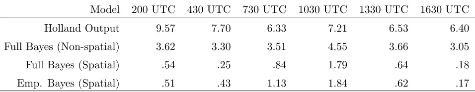
Table 3: RMSPE for V (m/s) based on 30 cross validation sites using the Holland model output
(fixed parameters), fully Bayesian prediction and the empirical Bayesian approach based on the non-spatial model (Model 1) and separable LMC model (Model 3).
Model 200 UTC 430 UTC 730 UTC 1030 UTC 1330 UTC 1630 UTC
Holland Output 9.57 7.70 6.33 7.21 6.53 6.40
Full Bayes (Non-spatial) 3.62 3.30 3.51 4.55 3.66 3.05
Full Bayes (Spatial) .54 .25 .84 1.79 .64 .18
Emp. Bayes (Spatial) .51 .43 1.13 1.84 .62 .17
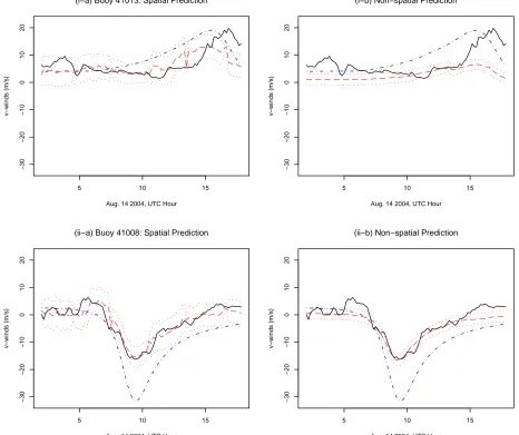
We also repeat the prediction of the v winds at the two buoys for the 96 time periods, this
time without using the observed winds at these two sites. Figure 4 shows the predicted values
under Model 3 (plots i-a and ii-a) and Model 1 (plots i-b and ii-b). The spatial model is still able
to better capture the variability in the winds when compared to the Holland model output. The
observed v winds fall outside the 95% posterior prediction intervals for plots i-a and ii-a 26% and
7% of the time periods, respectively. The non-spatial model also shows an improvement over the
Holland model output but the prediction intervals do not capture the observed values as often as
the intervals based on the spatial model. Thus there is a clear advantage in using the statistical
framework to estimate the Holland model parameters and the uncertainty in these parameters.
Furthermore, there is added value in incorporating a multivariate spatial covariance through the
stochastic component.
4.3 Storm Surge Prediction
The predicted wind fields are used as the input fields for the POM model to spin up and force
the ocean model for a time between August 14th hour 0 UTC and hour 18UTC. Observed water
levels were used from a series of coastal water level stations maintained by NOAA’s National Ocean
Service (NOS) Center for Operational Oceanographic Products and Services (CO-OPS). We have
hourly data at 7 coastal sites for Hurricane Charley for the surface water elevation in meters shown
Figure 4: Cross Validation Time Series Plots: Observedvwinds in m/s at each buoy in solid black for Aug. 14th 200-1750 UTC. The dashed and dotted line is the Holland output based on fixed parameter values (B = 1.9, Rmax= 46). The dashed line is the predicted values and the dotted lines are 95% credible intervals under (i-a), (ii-a) Model 3 and (i-b), (ii-b) Model 1.
(i−a) Buoy 41013: Spatial Prediction
Aug. 14 2004, UTC Hour
v−winds (m/s)
5 10 15
−30
−20
−10
0
10
20
(i−b) Non−spatial Prediction
Aug. 14 2004, UTC Hour
v−winds (m/s)
5 10 15
−30
−20
−10
0
10
20
(ii−a) Buoy 41008: Spatial Prediction
Aug. 14 2004, UTC Hour
v−winds (m/s)
5 10 15
−30
−20
−10
0
10
20
(ii−b) Non−spatial Prediction
Aug. 14 2004, UTC Hour
v−winds (m/s)
5 10 15
−30
−20
−10
0
10
and the effect of daily tidal levels to determine the change in water elevation that can be attributed
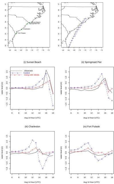
to storm surge. Figure 5 shows the observed water levels at each of these sites as Hurricane Charley
moves along the coast. The Sunset Beach site shows the greatest storm surge of 1.67 meters.
The dashed and dotted line shows the predicted water elevation at each site based on hourly
output of the Princeton Ocean Model under the original Holland wind forcings. Using the Holland
winds with fixed parameter values the ocean model tends to greatly overestimate the storm surge at
three of the four locations. The dotted line shows the predicted values using the statistically based
wind estimates,V=VH+V, where˜ V˜ is based on Model 3 (separable LMC). The prediction error is
reduced and at several of the sites these estimates tend to better capture the timing and magnitude
of the peak storm surge. However the model output based on the LMC winds underestimates the
greatest surge seen at the Sunset Beach site at 1600 UTC and in fact the Holland model better
predicts this peak value.
5
Discussion
Here we present a flexible hierarchical framework to incorporate observations from different data
sources with physical knowledge of hurricane surface wind fields. The multivariate spatial model
proposed here allows for cross dependency between the two wind components. We found that
including this dependency was important for estimation at the time periods when the hurricane
structure was more asymmetric. All of the spatial models assumed that the underlying univariate
processes of the stochastic residual component were Gaussian and stationary. Based on exploratory
analysis we found that the Gaussian assumption was reasonable. In terms of prediction the three
spatial models, Model 2, Model 3, Model 4, produced similar results and were able to produce very
accurate predictions when compared to the observed data. We also saw a clear improvement in
prediction when the Holland parameters were estimated using the statistical framework proposed
here (Model 1) when compared to the results based on “expert knowledge”.
Another approach to capture more complex spatial structures would be to allow for potential
Figure 5: Maps show the location of 7 coastal water elevation gauges and the track of Hurricane Charley on August 14th for hours 6 UTC to 18 UTC. Time series plots show observed water elevation at each site as a solid black line. The dotted line shows the predicted elevation using the predicted winds from the LMC statistical model to force the ocean model run. The dashed line shows the estimates when the ocean model is forced using the original Holland wind model.
−82 −81 −80 −79 −78 −77 −76 −75
30 31 32 33 34 35 36 37 Sunset Beach Springmaid Pier Charleston Fort Pulaski
−82 −81 −80 −79 −78 −77 −76 −75
30 31 32 33 34 35 36 37 5 6 7 8 9 10 11 12 13 14 15 16 17 18
6 8 10 12 14 16 18
−1.5 −1.0 −0.5 0.0 0.5 1.0 1.5
(i) Sunset Beach
Aug 14 hour (UTC)
water level (m)
−−−−−−−−−−−−− Observed
− − o − − o − − Control
−−−o−−−o−−−o−− Using LMC Winds
6 8 10 12 14 16 18
−1.5 −1.0 −0.5 0.0 0.5 1.0 1.5
(ii) Springmaid Pier
Aug 14 hour (UTC)
water level (m)
6 8 10 12 14 16 18
−1.5 −1.0 −0.5 0.0 0.5 1.0 1.5 (iii) Charleston
water level (m)
6 8 10 12 14 16 18
−1.5 −1.0 −0.5 0.0 0.5 1.0 1.5
(iv) Fort Pulaski
at times when the hurricane is less organized and either moving off the coast or making landfall.
As noted earlier, the proposed methodology can still be used in this case by allowing for the
underlying univariate processes to be non-stationary. Further analysis is necessary to test if this
added complexity would be needed.
Here we used empirical Bayes prediction for computational reasons but clearly a fully Bayesian
analysis provides slightly better coverage of the credible intervals. The cross validation analysis
shows that prediction results are similar under either approach. Also of interest would be to consider
a temporal component to allow for the evolution of the wind fields over time. For example, Wikle
et al. (2001) present a hierarchical spatio-temporal model applying a first-order Markov vector
autoregression model.
In applications such as storm surge prediction it is often unclear whether prediction errors are a
result of simplified or neglected physical processes used in the numerical model, inaccuracies in the
initial conditions or as was investigated here, errors in the forcing fields. It is likely the remaining
prediction errors in the storm surge application presented here are a result of a combination of
these factors. Thus changes in the ocean model itself may be necessary to reduce errors further.
For example, the ocean model can be run at a higher resolution for this region and coupled with
an inundation model that allows for flooding and drying in shallow coastal areas. Coastal ocean
prediction for hurricane applications remains a challenging problem since we must balance potential
improvement in estimation and prediction from a more sophisticated model and computational cost.
In terms of computational cost, the greatest cost of the methods presented here is from the Gibbs
sampling algorithm required for the estimation of the parameters of the statistical model whenever
HRD data is available. This step takes approximately fifty minutes for 1000 updates using the
WinBUGS software. However the prediction step using the empirical Bayes approach takes only
minutes to create the gridded wind inputs based on all available buoy data at ten minute intervals.
Thus after an initial lag when new HRD data becomes available it is possible to run the ocean
Acknowledgements: This study is supported by the National Oceanic and Atmospheric
Ad-ministration through the Carolina Coastal Ocean Monitoring and Prediction System (Caro-Coops)
Program, via a subcontract from the University of South Carolina. We greatly appreciate the help
and advice on the use of the ocean model application provided by members of the Coastal Fluid
Dynamics Laboratory headed by Dr. Lian Xie at North Carolina State University.
References
Banerjee, S., Carlin, B. P. and Gelfand, A. E. (2004).Hierarchical modeling and analysis for spatial
data. Chapman & Hall. New York.
Berliner, L. M., Royle, J. A., Wikle, C. K. and Milliff, R. F. (1999). Bayesian methods in the
atmospheric sciences. Bayesian Statistics 6 – Proceedings of the Sixth Valencia International
Meeting pp. 83–100.
Blumberg, A. F. and Mellor, G. L. (1987). A description of a three-dimensional coastal ocean
circulation model. in N. S. Heaps, ed., ‘Three-Dimensional Coastal Ocean Models’. American
Geophysical Union. Washington, D.C.. pp. 1–16.
Cripps, E., Nott, D., Dunsmuir, T. M. and Wikle, C. K. (2005). Space-time modelling of Sydney
Harbour winds. Australian and New Zealand Journal of Statistics 47, 3–17.
Ezer, T. and Mellor, G. L. (1997). Data assimilation experiments in the Gulf Stream region: How
useful are satellite-derived surface data for nowcasting the subsurface fields?. Journal of
Atmo-spheric and Oceanic Technology 14, 1379–1391.
Fuentes, M. and Raftery, A. (2005). Model evaluation and spatial interpolation by Bayesian
com-bination of observations with outputs from numerical models. Biometrics 61, 36–45.
Fuentes, M., Chen, L., Davis, J. M. and Lackmann, G. M. (2005). Modeling and predicting complex
space-time structures and patterns of coastal wind fields. Environmetrics 16, 449–464.
Gelfand, A. E. and Smith, A. F. M. (1990). Sampling-based approaches to calculating marginal
Gelfand, A. E., Schmidt, A. M., Banerjee, S. and Sirmans, C. F. (2004). Nonstationary multivariate
process modeling through spatially varying coregionalization (with discussion). TEST13, 1–50.
Holland, G. (1980). An analytic model of the wind and pressure profiles in hurricanes. Monthly
Weather Review 108, 1212–1218.
Houston, S. H. and Powell, M. D. (1994). Observed and modeled wind and water-level response
from tropical storm Marco (1990). Weather and Forecasting9, 427–439.
Houston, S. H., Shaffer, W. A., Powell, M. D. and Chen, J. (1999). Comparisons of HRD and
SLOSH surface wind fields in hurricanes: Implications for storm surge modeling. Weather and
Forecasting14, 671–686.
Hsu, S. A. and Yan, Z. (1998). A note on the radius of maximum wind for hurricanes. Journal of
Coastal Research 14, 667–668.
Large, W. G., Morzel, J. and Crawford, G. B. (1995). Accounting for surface wave distortion
of the marine wind profile in low-level Ocean Storms wind measurements. Journal of Physical
Oceanography25, 2959–2971.
Peng, M., Xie, L. and Pietrafesa, J. (2004). A numerical study of storm surge and inundation in the
Croatan-Albemarle-Pamlico Estuary System.Estuarine, Coastal and Shelf Science 59, 121–137.
Powell, M. D. and Houston, S. H. (1996). Hurricane Andrew’s landfall in South Florida. Part II:
Surface wind fields and potential real-time applications. Weather Forecast11, 329–349.
Powell, M. D., Houston, S. H. and Reinhold, T. A. (1996). Hurricane Andrew’s landfall in South
Florida. Part I: Standardizing measurements for documentation of surface wind fields. Weather
Forecast 11, 304–328.
Royle, J. A., Berliner, L. M., Wikle, C. K. and Milliff, R. (1999). A hierarchical spatial model for
constructing wind fields from scatterometer data in the Labrador Sea.Case Studies in Bayesian
Statistics Volume IV pp. 367–382.
Schmidt, A. M. and Gelfand, A. E. (2003). A Bayesian coregionalization approach for multivariate
Spiegelhalter, D. J., Best, N. G., Calin, B. P. and van der Linde, A. (2002). Bayesian measures
of model complexity and fit (with discussion). Journal of the Royal Statistical Society, Series B
64, 583–640.
Spiegelhalter, D., Thomas, A., Best, N. and Gilks, W. (1996). Bugs .5 Bayesian inference using
Gibbs sampling. Manual, version ii. MRC Biostatistics Unit, Institute of Public Health.
Cam-bridge, U.K.
Stein, M. L. (1999). Interpolation of Spatial Data. Some Theory for Kriging. Springer. New York,
N.Y.
Wackernagel, H. (1998). Multivariate geostatistics: An introduction with applications. Springer.
New York.
Wikle, C. K., Berliner, L. M. and Cressie, N. (1998). Hierarchical Bayesian space-time models.
Environmental and Ecological Statistics5, 117–154.
Wikle, C. K., Milliff, R. F., Nychka, D. and Berliner, L. M. (2001). Spatiotemporal hierarchical
Bayesian modeling: Tropical ocean surface winds.Journal of the American Statistical Association
96, 382–397.
Xie, L., Bao, S., Pietrafesa, L., Foley, K. and Fuentes, M. (2006). A real-time hurricane surface
wind forecasting model: Formulation and verification.Monthly Weather Review134, 1355–1370.
Xie, L., Pietrafesa, L. and Peng, M. (2004). Incorporation of a mass-conserving inundatoin scheme