A MODEL OF EVOLUTIONARY BASE SUBSTITUTIONS AND ITS APPLICATION WITH SPECIAL REFERENCE TO
RAPID CHANGE OF PSEUDOGENES*
NAOYUKI TAKAHATA AND M O T 0 0 KIMURA
National Insiitute of Genetics, Mishima, 411 Japan
Manuscript received February 2, 1981 Revised copy received May 18,1981
ABSTRACT
A model of evolutionary base substitutions that can incorporate different substitutional rates between the four bases and that takes into account unequal composition of bases in DNA sequences is proposed. Using this model, we de- rived formulae that enable us to estimate the evolutionary distances in terms of the number of nucleotide substitutions through comparative studies of nu- cleotide sequences. In order to check the validity of various formulae, Monte Carlo experiments were performed. These formulae were applied to analyze data on DNA sequences from diverse organisms. Particular attention was paid to problems concerning a globin pseudogene in the mouse and the time of its origin through duplication. W e obtained a result suggesting that the evolu- tionary rates of substitution i n the first and second codon positions of the pseudogene were roughly 10 times faster than those i n the normal globin genes; whereas, the rate in the third position remained almost unchanged. Application of our formulae to histone genes H2B and H3 of the sea urchin showed that, in each of these genes, the rate in the third codon position is tremendously higher than that in the second position. All of these observa- tions can easily and consistently be interpreted by the neutral theory of mo- lecular evolution.
R E C E N T developments in DNA-sequencing techniques ( MAXAM and GILBERT 1977; SANGER, NICKLEN and COULSON 1977), together with methods for amplifying gene copies in a bacterial plasmid, have made possible rapid deter- minations of DNA sequences of genes. Because data on DNA sequences are obtainable only from living organisms, it is necessary to develop mathematical models to estimate the number of evolutionary nucleotide substitutions through comparison of DNA sequences of homologous genes in related species.
Prior to a recent flood of data on nucleotide sequences, there already existed a large body of data on amino acid sequences in diverse organisms, and many mathematical models have been proposed to treat protein evolution in terms of amino acid substitutions, (see, for example, ZUCKERKANDL and PAULING 1965; FITCH and MARGOLIASH 1967; JUKES and CANTOR 1969; OHTA and
KIMURA 1971; NEI 1975 for review). However, for comparative studies of nucleotide sequences, different mathematical models have to be employed. Sev-
* Contribution No. 1354 from The National Institute of Genetics, Mishima, Shizuoka-ken, 411 Japan.
642 N. T A K A H A T A A N D M. K I M U R A
era1 authors have considered the problem of estimating the evolutionary distance of the homologous part of the genome between related species (JUBES and
CANTOR 1969; KIMURA and OHTA 1972;
MIYATA
andYASUNAGA
1980; HOLM- QUIST 1980; HOLMQUIST and PEARL 1980).Recently, KIMURA (1980; 1981) developed three different models that can partially incorporate different substitutional rates between four bases and ap- plied them to analyze data on various nucleotide sequences from several organ- isms. He showed that a preponderance of synonymous and other silent nucleotide substitutions is a general feature of molecular evolution and that this is consis- tent with the neutral theory
(KIMURA
1968; see KIMURA 1979 for review).In this paper, we extend the mathematical models of KIMURA (1980. 1981), and we derive appropriate formulae f o r estimating evolutionary distances in terms of the number of nucleotide substitutions per site. In addition to an an- alytical treatment, we used simulation methods to check the validity of the formulae and determine their range of applicability. This is necessarj- because formulae for estimating evolutionary distances generally do not have high resolving power when they are applied to evolutionarily distant organisms; they are accompanied by large error variances. Therefore, we conducted extensive Monte Carlo experiments in which the values of the parameters involved were greatly altered.
W e have applied our formulae to analyze actual data on nucleotide sequences. Particular attention was paid to the evolution of the globin pseudogene in the mouse ( NISHIOKA, LEDER and LEDER 1980;
VANIN
et al. 1980). Although similar analyses have recently been carried out by KIMURA (1980), PROUDFOOT andMANIATIS
(1980) and, in more detail, by MIYATA and YASUNAGA (1981 ),
we re-examined the problem to estimate the time of its origin and to discuss the evolutionary implications.M O D E L A N D A N A L Y S I S
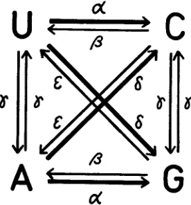
Let us consider a model of base substitutions, as shown in Figure 1, in which the four bases are represented by the letters U, A, C and G in terms of mRNA codes. The rates of base substitutions per unit time (say, year) between the four bases are designated by a,
8,
y, 6 and E . For instance, a! is the rate of transition-type substitutions from U to C or A to G, while
p
is the rate for the reverse direc- tions. The rates of transversion-type substitutions are denoted by y, 6 and E . In comparing two homologous sequences, there are 16 combinations of base pairs at each site. The possible combinations and their relative frequencies (prob- abilities) are listed in Table 1. They represent the expected relative frequenciesof their occurrence in two homologous sequences. For example, S (the sum of
Si’s) stands for the probability that the bases at a homologous site are identical and P (= 2P,
+
2P,) the probability of their showing transition-type differences, while Q (= 2Q1+
24,) and R (= 2R,4-
2R,) are the probabilities of transver- sion-type differences.BASE SUBSTITUTIONS I N EVOLUTION 643
FIGURE 1.-Scheme of base substitutions and their rates per unit time.
probabilities at time T
+
AT, using their probabilities at timeT ,
and the rates of base substitutions, where AT stands f o r a short time interval. Neglecting small quantities involving ( A T ) and higher order terms, we have, for example,U(Tl+AT) = (1
-
( a + S + y ) ~ T } U ( T ) +@ATC(T) +sATC(T) f y s l T A ( T ) . As seen from Figure 1, the first term in the right-hand side of this equation corresponds to the probability of no change, and the last three terms are the probabilities that U came from the remaining three bases during the short time interval AT.T h e
corresponding probabilities for other bases can be obtained in a similar manner, and we get the following set of ordinary differential equations by letting AT -+ 0;--__ m ( T ) - - - ( a
+
S+
y ) U ( T ) +,8C(T)+
E G ( T ) -I- y A ( T ),
dT
dT
d A ( T ) = - ( a
+
S f y ) A ( T )4-
,8G(T)4-
& ( T )4-
y U ( T ),
d C ( T ) = -(,8
4-
E+
y ) C ( T )+
a U ( T )+
S A ( T )+
y G ( T ),
dT
d G ( T ) - -(,8
4-
E4-
y ) G ( T )+
a A ( T )+
SU(T)4-
y C ( T ) .dT
Likewise, we can derive the equations for changes of probabilities of the base
TABLE 1
Types of nucleotide base pnirs occurring at homologous sites in two sequences and their probabilities (relative frequencies)
U C A G U C A G U A C G U G A C U C A G C U G A A U G C G U C A Types
SI S, S, S, 2P, 2P, 2Q, ZQ, 2R, ZR,
S P
Q
R644 N. TAKAHATA A N D M. KIMURA
pairs listed in Table 1 , although the procedures involved are more complicated. As a n example. let us consider the change of base pair UC. Noting that the prob- ability of UC is equal to that of CU. i.e., P,, we first get the probability of no change occurring in either nucleotide. This is [ l - ( a
+
y f ,)AT] [l -( p
+
y+
s ) A T ] , s3 that the contribution from this class is [ 1 - ( (Y f y+
& ) A T ] X [ l - ( p + y + S ) A T ] P , ( T ) . UC is also derived from UU and CC with prob- abilities [ 1 - ( a+
y+
F ) AT] AT and [ 1-
( ,L?+
y+
8 ) AT],L?AT. respectively. Then, the contribution from these classes is [ 1 - ( a+
y -k E ) AT]aATS, ( T ) f[ 1 -
( p
+
y+
8 ) AT]/?ATS2( T ) , Additional contributions come from pairs UAand GC with probabilities [ 1 - ( a
+
y+
&)AT] SATQ, ( T ) and [ 1 -( p
+
Y+
8 )~ T ] F A T Q , ( T ) , and also from pairs UG and AC with probabilities [I - ( (Y f y
+
E ) A T ] y A T R , ( T ) and [ 1 -( p
+
y+
6 ) AT] y A T R , ( T ).
Combining all these contributions, and neglecting (AT)' and higher order terms, as before, we haveP,(T f AT) = [ l - ( a +/3
+
2 y f 8+
E ) A > ' ] P , ( T )f
a A T S , ( T )Continuing these calculations for other base pairs and taking the limit A T -+ 0,
we get a complete set of differential equations (equations 1). It is interesting to note that a more convenient derivation of equations (1 ) is possible if we use the differential equations for U ( T ) ,
A ( T ) ,
C ( T ) and G ( T ) and combine themthrough relationships such as
P , ( T ) = U ( T ) C ( T ) for the case of the UC pair. This is true because bases in one species change independently €rom those in other species. W e can verify by direct calculation that both derivations give the same set of equations. Thus,
we obtain a complete set of differential equations as follows:
d S 1 ( T ) 1 - 2 ( a
f
yf
S)S1(T) f 2 P P 1 ( T ) -t 2 y Q 1 ( T ) f 2ER1(T)d S z ( T ) = - 2 ( p
+
y+
E ) S ~ ( T )+
2aP1(T)
+
2 y Q , ( T )+
2SR2(7')3 2
= - 2 ( af
y f S ) S , ( T ) f 2/3P2(T)+
2yQ1(T)+
2ER?(T)d s 4 ( T ) = - 2 ( p
+
y+
E ) S 4 ( T )+
%P,(T)+
2yQn(T)+
26R1(T)d P 1 ( T ) = -(a
+
P
f 27+
6+
E ) P l ( T ) $- a S , ( T ) -f P S ? ( T ) f /3ATS,( T )+
SATQ, ( T )+
EATQ,( T )+
y A T { R i ( T ) fRL
( T ) } edU(T) and
d C ( T ) +C(T)--- dT = U ( T ) ___
dPi ( T )
dT dT
dT
dT
dT
dT
dT
+
6 Q l ( T )
+
E Q ~ ( T ) -k y [ R I ( T )+
Rz(T)I(1) d P z ( T ) = -(a f
p
+
27+
6+
E ) P z ( T )+
IrS,(T)+
PS,(T)+
SQ,(T) f ~ Q 2 ( 7 ' )+
y [ R i ( T ) + R 2 ( T ) IdT
d Q 1 ( T ) = - 2 ( a
+
y+
~ ) Q , ( T )+
Y [ S , ( T )+
s . , ( T ) I
+
E [ P ~ ( T ) + P 2 ( T ) ] f P [ R i ( T ) + R r ( T ) IA
BASE SUBSTITUTIONS I N EVOLUTION 645.
d R 1 ( T ) = -(a f
p
+
2yt
8f
E ) R l ( T ) f8Si(T)
f ESI(T)+
y [ P i ( T )+
P2(T)I+
+
PQ2(T)dT
d R z ( T ) = -(a
+
p
+
2y+
8+
E ) R , ( T )+
8S,(T)+
ESZ(T)+ y [ P , ( T ) +P2(T)I +aQi(T) + P Q 2 ( T ) .
dT
To solve equations ( 1 )
,
we define six variables1
( 2 ) X + ( T ) = S i ( T ) + S s ( T ) 2Q1(T)Y , ( T ) = S Z ( T ) t S , ( T )
*
2Q2(T)Z , ( T )
= P ( T )*
R ( T ) ,where we take the same sign for the subscripts of X , Y and 2 as that in the right- hand side. Then, from ( 1 ), we can derive two sets of equations.
x+
(TI -2(a+
8 ) 0z+
( T ) 2(a+
8 ) 2 ( p+
E ) -(a+
- ( Y + ( T ) ) = ( dT 0 - 2 ( P + & ) l Y f 8and
I n these equations, the transformation matrices have a common form
( 5 ) - ( c + d )
9
.
-2c 0
M = ( 0 -2d
2a 2b
Note that a = c and b = d hold in (3). As we can easily calculate the eigenvalues and projection operators for the matrix of ( 5 ) , we can solve the initial value problems of equations ( 3 ) and (4). Let hi’s (
(i
= 1,2 and 3) be the eigenvaluesand pi’s be the corresponding projection operators. Then, we have
hl = - ( c
+
d ) , h2 = - (c+
d - g ) and h, = - ( c+
d+
g ) : (6)and
2ab -2b2 -b(d-c)
2ab a(d-c)
646 N. TAKAHATA A N D M. K I M U R A
4ab ( d - C ) (d-c+g) f 2 a b 2b2
2a‘ (d-c) (d-c-g) f 2 a b -a ( d - c - g ) 2a (d-cfg) 2b ( - d f c f g )
4ab
( d - c ) (d-c-g) +2ab 2bZ
P3 =
2gz
2a2 ( d - c ) (d-cfg) f 2 a b -a( d-c+g)2a ( d - c f g ) 2 b ( d - ~ - g )
where g = d ( d - c ) ~
+
4ab.arbitrary initial condition of X (0). Thus,
By using these formulae, we obtain the solutions X ( T ) at time T under a n
(8)
X ( T ) = {eXFPl f eX,T”, -k eXPp3)X ( 0 )
where
X(
) is a column vector that can be either ( X + ,Y + ,
2,) or ( X - . Y-, 2-) t , in which the superscript t denotes the transpose.We assume that the frequency (U) of U
+
A does not change with time, andalso ihat U ( T ) = A ( T ) and C ( T ) = G ( T ) for all T. Then, S i ( T ) , P i ( T ) ,
Qi
( T ) and Ri ( T ) can all be expressed in terms of X ,
(7’)
,
Y , ( T ) and Zr ( T ).
The evolutionary rate of base substitutions per unit time isk r ( a + y + 6 ) W f ( p + y + E ) ( 1 - 0 ) ) (9)
(9a) or
k
7 f %I( 1 - W) (.Y fp
+
6f
E ).
These equations are derived from the consideration that
U
or A each with the irequency 0 / 2 changes to the other bases at the rate of a f y+
6 , and C or G each with (1 - 0 ) / 2 changes at the rate of ,8+
y f E . Note that we have w =(P
f E ) /(a
+
,8 4- 6 f E ) . Therefore, the expected number of substitutions per site between two species with divergence time T i s given byK = 2 T k .
If we use formula (9a) for k, then
K =2yT +40(1 - 0 ) ( a +/3 f 6 f E ) T . ( 1 0 ) Before deriving an expression for
K
in terms ofX , ,
Y , and Z , , we shall ob- tain the explicit expression for the eigenvalues and the functional forms of those quantities under the assumption of the steady state of U f A content. As the initial conditions are now( 1 1 )
X,(O) = (a, 1 - W , O ) f
for both cases, the solutions for
X+
( T ) are expressed in a simple form,X + ( T ) =U{,+ ( 1 -w)eV}
Y + ( T ) = ( 1 - 0 ) ( 1 - 0 + + V )
BASE SUBSTITUTIONS I N EVOLUTION 647
where
A o . = - 2 ( a + p f S + E )
.
(13)On the other hand, the eigenvalues of equation
(4)
areA 1 = -(,a
+ p
+
6 + E+
4y) A, = A I + gk3 = A 1
-
gwhere g 2 = { a + S - ( @ + ~ ) } ~ + 4 ( a - 6 ) ( @ - ~ ) . Using ( 7 ) and
(le),
the solutions forX-(
T ) are, for g # 0,1
X - ( T ) =- [2b{aw-b(1 - - 0 ) } e V ’ + {.$-0++’(l - - 0 ) } e V
gz
+
{ 7-0+
b2 ( 1 - 0 ) } e V ] 1Y - ( T ) =- [-2a{aw-b(1 - - w ) } e X 1 * f {a%
+
q ( 1 - -0))eVg L
+{a2-0+.$(1 -W)}eX3*]
1
2-( T ) =
-
[-2 ( d - c ) {ao - b (1 - 0 ) }eX,*+
{ a ( d-
c+
g ) -0g’
- b( d - c - g ) ( 1 - -0) }ehT
+
{ a ( d - c-
g ) m- b ( d
-
c+
g ) ( 1-
-0)}exs*]
in which u = a - 6 , b = p - E , c = a f 6 + 2 y , d = p + E + 2 y , [ = 1 / ( ( d - c )
(d - c
+
g ) +ab and 7 = 1/ ( d - c) ( d - c - g )+
ab. In this case. however, it does not seem feasible to derive a simple formula for 2A,T = ( A 2+
A,)T = -2( a
4-
p
4- 6 -k E+
4y) as a function ofX-(T)
and Q.A great simplification is possible if we assume that 6 = Ba and E = 8~3, where B is a constant. Then, equations ( 1 5 ) are much simplified (see 15a below), al- though equations (12) remain the same. Furthermore, 2yT in (10) can be ex- pressed in terms of
X - ( T ) ,
Y _ ( T ) , Z ( T ) and -0, which can be estimated fromobservations. The solutions for X ( T ) become, for a #
p
and 8 # 1,where -0 =
-
Note that, under the above assumption, if a =p ,
the modelreduces to the “three-substitution-type” (3ST) model of KIMURA (1981). Using equations (15a), we get
648 N. TAKAHATA A N D M. K I M U R A
Combining this with equations ( 12) and (13), we get
X ( T ) Y . ( T ) -
(w)]
o ( l - 0 ) -
(--
z+
( T I )I-
2?
and therefore we obtain a n appropriate equation for
K
as follows.-
or more explicitly
7 ( 1 8a)
where w is the fraction of the sum of two bases
U
and A, and SI, etc., are as defined in Table 1. I n addition, we can estimate the unknown parameter 0 b y using the relationship3
(S,
f
S,f
2Q1)
(S,4-
S, -24,)
-
(P-A)”
2-
“(1 - w )
1
4
K = - - 1 n
while the ratio of /3 to change with time and that
can be determined from the assumption that w does not
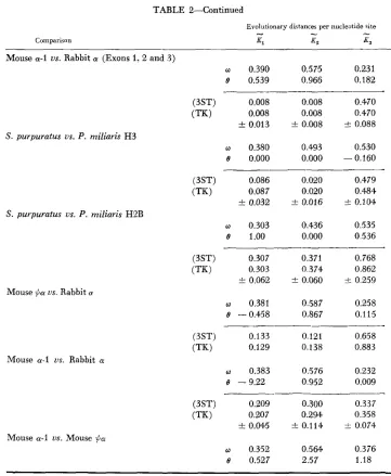
Formula (19) may be verified by substituting equations (15a) for the right- hand side of equation (19), noting a t the same time equations (2). Estimated evolutionary distances (denoted by K ) for several comparisons are shown in Table 2 together with values of 6 and The table also contains the estimates of the standard error of K that were obtained using a procedure similar to the one used by KIMURA (1980,1981) but assuming that the estimation of Cr) is not accom-
panied by sampling error. It is also based on the assumption of a multinomial distribution of the variables in the right-hand side of (18). This seems to give a good estimate in the light of the results of Monte Carlo experiments.
-
-
M O N T E CARLO E X P E R I M E N T S
BASE SUBSTITUTIONS I N EVOLUTION
TABLE 2
649
Euolutionary distances per nucleotide site at the first, second and third codcn position estimated b y using the 3ST and the present model (TK)
Comparison
Erolutionary distances per nucleotide site
-
-
-
Kl K 2 K ,
(3ST) 0.300
(TK) 0.299
f 0.044
Chicken /3 us. Rabbit p
w 0.384
0 0.489 (3ST) 0.265
(TK) 0.269
i 0.038
0.195 0.636 0.237 0.691 f 0.037 i 0.160 0.637 0.267 1.048 - 0.079
.__-__--
0.177 0.531 0.178 0.692 f 0.032 f 0.121 H u m a n us. Rat pregrowth hormone
w 0.430 0.609 0.258
e 0.592 0.135 0.468
(3.w 0.182 0.274 0.947
(TK) 0.1 78 0.289
i 0.273 f 0.104 ‘32 H u m a n us. Rat insulin C peptide
w 0.081 0.581 0.226
e 2.63 0.821 1
.oo
--_-
(3ST) 0.040 0.000 0.461
(TK) 0.042 0.000 0.786
f 0.026 i 0.019
*
0.300 H u m a n us. Rat insulin A+
B peptidew 0.480 0.628 0.275
6 0.964 1
.oo
0.535(3ST) 0.160 0.127 0.427
(TK) 0.171 0.135 0.463
i 0.031 i 0.030 f 0.080 Rabbit p us. Mouse p
61 0.373 0.6% 0.339
e 0.954 0.757 0.398
(3ST) 0.600 0.437 0.903
(TK) 0.600 0.51 7 1.29
i 0.087 f 0.062 f 1.05 Rabbit 01 us. Rabbit p
w 0.389 0.633 0.234
e 0.071 1.09 0.290
(3ST) 0.124 0.115 0.544
(TK) 0.126 0.131 0.774
650 N. TAKAHATA AND M. KIMURA
TABLE 2-Continued
Comparison
Evolutionary distances per nucleotide site
-
-
-
El K? 4
Mouse a-1 us. Rabbit a (Exons 1 , 2 and .3)
w 0.390 0.575 0.231
e 0.539 0.966 0.182
(3ST) 0.008 0.008 0.470
0.008 0.008 0.470
f 0.013 t 0.008 ? 0.088 ____
--
S. purpuratus us. P. miliaris H3
w 0.380 0.493 0.530
e O.OOO 0.000 -0.160
(3ST) 0.086
(W
0.087t 0.032
w 0.303
S. purpuratus us. P. miliaris H2B
e 1.00
Mouse +a us. Rabbit O/
Mouse a-1 us. Rabbit (Y
Mouse a-I us. Mouse pa
(3ST) 0.307
(TK) 0.303
t 0.062
0.020 0.479 0.020 0.484
+- 0.016 i- 0.104 0.436 0.535
0.000 0.536
0.371 0.768 0.374 0.862
+- 0.060 i 0.259
--
w 0.381 0.587 0.258
e - 0.458 0.867 0.115
(3ST) 0.133 0.121
(TK) 0.129 0.138
w 0.383 0.576
e - 9.22 0.952
(3ST) 0.209 0.300
--_
(TK) 0.207 0.294
t 0.045 t 0.114
o 0.352 0.5M
e 0.527 2.57
0.658 0.883 0.232 0.009 0.337 0.358 i: 0.074
___-
0.376 1.18
First, we prepared a random nucleotide sequence to be used as a commmon an- cestor. It consisted of n sites, with frequencies of U, A. C and G being given by 0/2,0/2, ( 1
-
0 ) / 2 and ( 1 - O ) /2. From this sequence, two descendent sequencesBASE SUBSTITUTIONS I N EVOLUTION 65 1
number of nucleotide substitutions,
K ,
was monit,ored by summing the actual numbers of substitutions observed until a given time T. On the other hand, the expected number of nucleotide substitutions overT ,
as denoted byK E ,
was calcu- lated by 2kT for a given value ofk.
Note that, strictly speaking, K E is different from K , although no significant differences between these two were observed in the simulations experiments. We also observed the relative frequencies of the various classes in Table 1 at specified times and calculated the estimtaed evolu- tionary distances using equation (1 8) or (1 8a). In a similar way, we obtained the estimate K J c = --
In( 1 - -h) as a reference point; where h is the fractionof different sites between two nucleotide sequence; (see JUKES and CANTOR 1969; KIMURA and OHTA 1972). These processes were repeated 100 times, as- suming n = 100. Each quantity of concern was obtained by taking the average. The results are illustrated through Figures 2 to 4. As typical situations, we assigned the parameter values similar to the ones derived from comparisons of DNA sequences of exons 1 and 2 in the mouse and the rabbit #@-globin genes, to- gether with a mouse pseudogene. The parameters are determined separately at different codon positions. Figures 2, 3 and
4.
respectively, represent situations at3 4
4 3
-
1.2
-
1.1
-
w1.0-
:9-
Z
I
.8-a
5 . 7 -
tu
ca .- .6-
5 .5-
Ls
CI
3
e
= 0.1 2U= 0.37
ro= 0.59d
r = 0 . 1 7 d
Evolutionary Distance K
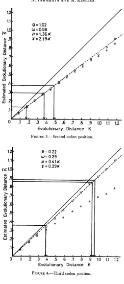
FIGURE 2 to 4.-Relationship between the actual evolutionary distance K and the estimated evolutionary distance K based on the formula (18) (the broken lines). Th- solid lines represent
K = K. The parameters used i n these figures are determined by taking the average for the data on nucleotide sequences of the ,(li globin gene and the a pseudogene (a3) of the mouse, and the
a-globin gene of the rabbit. FIGURE 2: First codon position.
-
652 N. TAKAHATA A N D M. KIMURA
1.2
-
1.1
-
e
= 1.02w = 0.58
l J . 0
-
P = 1 . 3 6 dT = 2.1 9d
8
.9-J 8 -
is
2 c
U)
.7
-
.6-
rrr .- c
3
.5-I3
I I I I , ,
0 .l .2 .3 .4 .5 .6 .7 .8 .9 1.0 1.1 1.2
Evolutionary Distance K
FIGURE 3.--Second codon position.
BASE SUBSTITUTIONS I N EVOLUTION 653
the first, second and third positions of codons within the above two exons. The abscissa stands for the actual evolutionary distance K (in terms of the number of base substitutions)
,
while the ordinate represents the estimated evolutionary distance K . Because the difference between K and K , turned out to be quite small in all experiments, we will not discriminate between them. Estimates obtained by using equation (18) are marked by open circles, while those estimated by using the fomula of JUKES and CANTOR (1969) are indicated open triangles. It is evident from Figure 3 that both sets of estimaies are close to each other when 6‘ is near 1 and 0 is about 0.5 and that they need appropriate corrections whenK
is large. Such a discrepancy for the second codon position seems to have been caused by the relatively high transversion type substitution rate y assumed. On the other hand, when 6’ and o are, respectively, less than 1 and 0.5, marked differencebetween the two sets of estimators occur (see Figures 2 and
4).
Fortunately, equa- tion (18) provides good estimates of the actual evolutionary distance if K does not exceed unity, and the linearity is almost completely preserved in this range ofK
values. The simulation experiments show that the present formula (18) is useful, especially when the rates of transversion-type subsiitutions are low and the fre- quencies of two classes of bases differ greatly from each other. Although not per- fectly proven, if the real pattern of base substitutions is something like this. the present method is the most accurate, followed by the 3ST (KIMURA 1981) and
JUKES and CANTOR methods. On the other hand, if substitution rates are equal in all directions, all three methods of these give almost the same result.
Note that cases arise in which we cannot estimate the evolutionary distances from these formulae. This occurs when arguments of logarithms become zero or negative. Such situations should occur frequently when a great many substitu- tions are involved. Because we excluded such-inapplicable cases from our calcula- tions, the estimated evolutionary distance K gives a n underestimate for
K .
I n some cases, the fraction of such inapplicable cases for formula (1 8) became more than 50% if K 2 1. When we analyze actual data, this difficulty often arises if we compare the sequences in which many substitutions have occurred. One example is afforded by the third position of codons in the C peptide of insulin when compar- ison is made between human and rat (see Table 2). Such a problem arises because the true nature of substitutional processes is stochastic; whereas, our present treat- ment is deterministic. As the number of nucleotide sites actually compared is finite, sometimes less than 100, the small sample size creates a large sampling error. Particularly, when K>
2, no estimator seems to provide good information on the actual evolutionary distance, as simulation experiments show. W e also note that in such casesK
has a very large error variance.-
-
RESULTS A N D DISCUSSION
Using equation (1 8 ) , we calculated the evolutionary distances between various DNA sequences, as shown in Table 2. This table also contains evolutionary dis- tances estimated using the “three-substitution-type” (3ST) model of KIMURA
654 N. T A K A H A T A A N D M. K I M U R A
and E = 6 in Figure 1 )
.
It can be seen from this table, that equation (18) often provides larger estimates than the corresponding estimates obtained from the 3ST model. Particularly, when the estimated value of 0 from equation (19) is small and that of from (20) differs noticeably from 0.5, the discrepancy between the two sets of estimates becomes large. Such a dependence of equation (18) onw seems to represent a favorable property as an estimator of evolusionary dis-
ance because, as pointed out by Kimura (1981 ), the U and A content, particularly at the third position of codons, is often much less than 0.5. For instance, the value of w is about 0.23 at the third codon positions in rabbit (Y and /3 globins. This bias often results in unreliable estimates of the evolutionary distance, as we men- tioned before.
On the other hand, the value of 0 is quite sensitive to changes of observed values
of various classes involved in equation (19). In most cases, 0 is less than unity, but, in some cases, it happens to be negative or exceed unity. The estimated value of 0 for each case may not be reliable, but the results suggest that transition-type substitutions can occur more frequently than those of transversion types (i.e.,
from U to G and A to C. or uice uersa)
.
It is fortunate that equation (18) does not contain 0.It may be clear from Table 2 that evolutionary base substitution is faster (roughly 2.5
-
5.9 times) at the third position of codons than at the second posi- tions in the functional globin genes. This characteristic is particularly conspicuous in histone genes. The ratio per site of the rates of third to the second positions is about 59 for the comparison of S. purpuratus and P. miliaris H3 sequences, while it is about 24 for the H2B sequences in the same comparison (for data, see SURES, LOWRY and KEDES 1978; SCHAFFNER et al. 1978). These species probably di- verged between 6 X 10' and 16 x 10: years ago (DURHAM 1966; KEDES 1979); therefore, the ratek,
per site per year is (1.5-
3.9) x for the H3 sequences and (1.5-
4.0) x for the H2B sequences. These values are very similar; moreover, the ratesk,
estimated for other genes using several other comparisons show roughly the same values. For example, we have 4.3 x for the human and rat pregrowth hormone comparison (with the divergence time T = 8 x lo7 years) and 1.2 x for the chicken and rabbitp
globin comparison ( T = 3 x1 Os years). In some cases, formula (1 8) gives 1.4 to 1.7 times higher estimates for
k,
than does the 3ST model. but whether or not the model can decrease the esti- mated variance ofk,
is still uncertain until more data are available. The rough equality of the evoluticnary rates at the third position of codons among genes is in sharp contrast to wide differences of the rate at the second position, where most substitutions alter amino acids. At any rate, we can confirm the conclusion ofKIMURA (1980, 1981) and MIYATA, YASUNAGA and NISHIDA (1980) that the rates of nucleotide substitutions at the third position of codons are not only very high but also roughly equal to each other between genes even when amino acid altering substitutional rates are quite different.
BASE SUBSTITUTIONS I N EVOLUTION
655
normal a-globin genes, including the noncoding regions, have also been deter- mined in the mouse and the rabbit (see KONKEL, MAIZEL and
LEDER
1979;HARDI-
SON et aZ. 1979, and references therein). Thus, we can compare DNA sequences of these three genes. Our aim is to estimate the time of occurrence of duplication leading to the a pseudogene in the mouse line and the relative evolutionary rates at each codon position in the pseudogene relative to those in the normal a-globin genes. Although several models concerning the appearance of pseudogenes are conceivable (see for example PROUDFOOT and MANIATIS 1980; MIYATA and YASUNAGA 1981; LI, personal communicatim), we assume here a simple one.
Let us assume that the duplication occurred Td years ago, and thereafter a duplicated gene became “dead” and started to evolve at the rate k’i instead of ki, where i (= 1 , 2 or 3) denotes the codon position. At the incipient stage, the mouse population must have been polymorphic with respect to the number of a-globin genes per individual. However, it is likely that the duplicate gene could accumu- late mutations at a higher rate than the normal gene, due to its-multiplicity. Let
To be the divergence time of the mouse and the rabbit, and let Ki ( X
-
Y ) be the evolutionary distance in the ith_ codon position of homologous genes between speciesX
and Y . For example,K i
(M$a-Ra) denotes the evolutionary distance in the ith position between the mouse LY psEdogene and the rabbit a gene. I n the following study, we make no correction for K and compare only the part including exon 1 and 2, excluding the exon 3 region from the calculation because of an un- usual characteristic of this region, as pointed out by MIYATA and YASUNAGA (1981). Then, Td and ki’, relative to To and ki. can be calculated for each codon position by-
-
-
T d - Ki(Ma-M$a)
-
Ki(M$a--Ra) K ~ ( M ( Y - R o L )-- ____
T
-
Ki
(Ma-Ra) 1 0and
--
-
-
ki K ~ ( M ~ - M + ~ ) - K ~ ( M $ ~ - R ~ )
+
K ~ ( M ~ - R ~ )
.Substituting the values of Table 2 in the above equations, the ratios of Td/To are respectively, 0.26, 0.42 and 0.43 for the first, second and third codon positions, while k,‘/k, = 11.5, k,’/k2 = 13.9 and k3‘/k3 = 0.9. Roughly speaking, this means that the duplication responsible for the mouse (Y pseudogene occurred about (0.3
-
0.4)T0 years ago. If we take 8.0 x 10’ as To, Td becomes about 20-
30 million years. On the other hand, the rates in the first and second positions in the pseudo- gene turn out to be roughly 10 times faster than those of normal genes; whereas, the rate in the third positions remain unaltered. The estimated values of 2k,’T,656 N. 'I'AKAHATA A N D M. K I M U R A
tionary distance. Considering the fact that estimated values of
k,
andk,'
are similar, the latter might be more probable in the light of the results of Monte Carlo experiments. W e could make some correction for the values of K based on Monte Carlo experiments, but we did not take such a n approach here because it seemed unlikely that we can get more precise estimates of these values because of the inevitable large sampling errors.I n the above analysis, we have tacitly assumed that the (Y pseudogene is fixed in the mouse population. In fact, it is likely that several million years are sufficient for such a nonfunctional pseudogene to become fixed in a population (see MARU- YAMA and TAKAHATA 1981 ; TAKAHATA 1981). Therefore, it is highly probable that the pseudogene is fixed in the mouse population. This conclusion, however, is tentative in the sense that we ignored the effect of recurrent unequal crossing over. As pointed out by OHTA (1981), it is possible that unequal crossing over plays a prominent role in the evolution of duplicate genes, even when a small number of them are tightly linked (i.e., multigene family of small size). If un- equal crossing over occurs frequently in the course of evolution, the fixation of a pseudogene at a specific locus may be considered transient. However, a prelimi- nary study incorporating such a mechanism still supports the view that all indi- viduals carry a pseudogene in their genome for several million years, although its location on a chromosome may vary from individual to individual or in time,
(the details will be published elsewhere).
We conclude that a duplicate gene leading to the (Y pseudogene in the mouse line was introduced 20
-
30 million years ago by unequal crossing over and became fixed in the population several million years after the duplication oc- curred, and that many nucleotide substitutions have accumulated at a high rate, irrespective of codon position, due to the loss of selective constraints.-
We thank K. AOKI for his helpful comments in composing the manuscript and T. OHTA for stimulating discussion.
L I T E R A T U R E C I T E D
DURHAM, J. W., 1966 Echinoides. pp. 270-295. In: Treatise on Inuetebrate Paleontology, Part FITCH, W. M. and E. MARGOWASH, 1967 Construction of phylogenetic trees. Science 155: 279-
HARDISON, R. C., E. T. BUTLER 111, E. LACY, T. MANIATIS, N. ROSENTHAL and A. EFSTRATIDIS, 1979 The structure and transcription of four linked rabbit P-like globin genes. Cell 18:
1285-1 297.
HOLMQUIST, R., 1980 Evolutionary analysis of cy and /3 hemoglobin genes by REH theory under
the assumption of equiprobability of genetic events. J. Mol. Evol. 15: 14Q-159.
HOLMQUIST, R. and D. PEARL, 1980 Theoretical foundations for quantitative paleogenetics. 111. The molecular divergence of nucleic acids and proteins for the case of genetic events of unequal probability. J. Mol. Evol. 16: 21 1-267.
JUKES, T. H. and C. H. CANTOR, 1969 Evolution of protein molecules. pp. 21-123. Mammalian
Protein Metabolism. Edited by H. N. MUNRO. Academic Press, New York.
KEDES, L. H., 1979 Histone genes and histone messengers. Ann. Rev. Biochem. 48: 837-870.
U , Echinodermata 3. Edited by R. C. MOORE. Univ. Kansas Press, Lawrence, Kansas.
BASE SUBSTITUTIONS I N EVOLUTION 65 7
Evolutionary rate at the molecular level. Nature 217: 624-626. -, The neutral theory of molecular evolution. Scientific American 241(5): 98-126.
1980 A simple method for estimating evolutionary rates of base substitutions
-,
On estimation of evolutionary distances between homologous nucleotide sequences.
On the stochastic model for estimation of mutational distance
The evolution and sequence comparison
Numerical studies of the frequency trajectories in the
A new method for sequencing DNA. Proc. Natl. Acad. Sci.
Molecular evolution of mRNA: A method for estimating evolutionary rates of synonymous amino acid substitutions from homologous nucleotide se- quences and its application. J. Mol. Evol. 16: W-36. -- , 1981 Rapid evolving mouse alpha globin-related pseudogene and its evolutionary history. Proc. Natl. Acad. Sci. U.S. MIYATA, T., T. YASUNAGA and T. NISHIDA, 1980 Nucleotide sequence divergence and func- NEI, M., 1975 MoZecuZar Population Genetics and Evolution. North-Holland Publishing Com- NISHIOKA, Y., A. LEDER and P. LEDER, 1980 Unusual a-globin-like gene that has clearly lost OHTA, T., 1981 Genetic variation in small multigene families. Genet. Research 37: 133-149. O H T ~ , T. and M. KIMURA, 1971 On the constancy of the evolutionary rate of cistrons. J. Mol.
Evol. 1: 18-25.
PROUDFOOT, N. J. and T. MANIATIS, 1980 The sbucture of a human cy-globin pseudogene and its relationship to cy-globin gene duplication. Cell 21: 537-544.
SANGER, F., S. NICKLEN and A. R. COULSON, 1977 DNA sequencing with chain-terminating inhibitors. Proc. Natl. Acad. Sci. U.S. 74: 4563-4567.
SCHAFFNER, W., G. KUNZ, H. DAETWYLER, J. TELFORD, H. 0. SMITH and M. L. BIRNSTIEL, 1978 Genes and spacers of cloned sea urchin histone DNA analyzed by sequencing. Cell 14:
655471.
SURES, I., J. LOWRY and L. H. KEDES, 1978 The DNA sequence of sea urchin (S. pupuratus)
H2A, H2B and H3 histone coding and spacer regions. Cell 15: 1033-1044.
TAKAHATA, N., 1981 On the disappearance of duplicate gene expression. In: Molecular Euolu- tion, Protein Polymorphism and The Neutral Theory. Edited by M. KIMURA. Japan Scien- tific Societies Press, Tokyo. ( I n press).
VANIN, E. F., G. I. GOLDBERG, P. W. TUCKER and 0. SMITHIES, 1980 A mouse a-globin-related pseudogene lacking intervening sequences. Nature 286 : 222-226.
ZUCKERKANDL, E. and L. PAULING, 1965 Evolutionary divergence and convergence in proteins.
pp. 97-166. In: Evolving Genes and Proteins. Edited by V. BRYSON and H. J. VOGEL. Academic Press: New York and London.
Corrsponding editor: M. NEI KIMuR~, M., 1968
1979
-,
through comparative studies of nucleotide sequences. J. Mol. Evol. 16: 111-120. 1981
Proc. Natl. Acad. Sci. U.S. 78: 454-458.
between homologous proteins. J. Mol. Evol. 2 : 87-90. of two mouse chromosomal P-globin genes. Cell 18: 865-873.
process of fixation of null genes at duplicated loci. Heredity 46: 49-57. U.S. 74: 560-564.
KIMURA, M. and T. OHTA, 1972
KONKEL, D. A., J. V. MAIZEL, JR. and P. LEDER, 1979 MARUYAMA, T. and N. TAKAHATA, 1981
MAXAM, A. and W. GILBERT, 1977 MIYATA, T. and T. YASUNAGA, 1980
78: 450-453.
tional constraint in mRNA evolution. Proc. Natl. Acad. Sci. U.S. 77: 7328-7332.
pany: Amsterdam, Oxford.