EXCURSIONS ALONG THE INTERFACE BETWEEN DISRUPTIVE AND STABILIZING SELECTION

EXCURSIONS ALONG THE INTERFACE BETWEEN DISRUPTIVE AND STABILIZING SELECTION

JOSEPH FELSENSTEIN

Department of Genetics, University of Washington, Seattle, Washington 98195

Manuscript received May 4, 1978 Revised copy received March 23, 1979

ABSTRACT

When a polygenic character is exposed to natural selection in which the curve giving fitness as a function of phenotype is a mixture of two Gaussian (normal) curves, the population may respond either by evolving to a spe- cialized phenotype near one of the two optimum phenotypes, o r by evolving t o a generalized phenotype between them. Using approximate multivariate normal distribution methods, it is demonstrated that the condition for selection to result in a specialized phenotype is that the curve of fitness as a function of breeding value be bimodal. This implies that a specialized phenotype is more likely to result the higher is the heritability of the character. Numerical iterations of four-locus models and algebraic analysis of a symmetric two-locus model generally support the conclusions of the normal approximation.

D I S R U P T I V E selection has been subject of much controversy in population genetics, mostly concerned with its alleged powers of maintaining poly- morphism or bringing about sympatric speciation (MATHER 1955; MAYNARD SMITH 1962). However, very little theoretical work has been done on disruptive selection. This has resulted from a concentration on types of natural selection that might maintain polymorphism, and also perhaps from a realization that dis- ruptive selection is likely to be rare in nature.We may define disruptive selection as that in which fitness rises steadily as the phenotype departs from a pessimum value. In nature, whenever we are not dealing with a primary component of fitness, a sufficiently extreme phenotype will nearly always cause a decrease in fitness.

Disruptive selection is thus most likely to be encountered in nature in combina- tion with stabilizing selection, such that if fitness at first rises as the phenotype de- part from a pessimum value, it will ultimately begin to decline again as the departure is made larger. There will then be two peaks in a plot of fitness versus phenotype, with a valley between them. We may consider this case to involve a combination of disruptive and stabilizing selection; alternatively, we may con- sider this to be selection for two optimum phenotypes at the same time. DICKIN-

SON and ANTONOVICS (1972) have summarized the results of deterministic com-

7 74 JOSEPH FELSENSTEIN

graphic subdivisions of the population. Since geographic subdivision affects the outcome substantially, their results cannot be directly compared to those in this paper.

This paper treats the case of simultaneous selection for two phenotypic optima, when the phenotype is determined additively by a number of loci. The selection is assumed to be both density- and gene-frequency-independent, with a constant fitness for each phenotype. While the mathematical treatment may seem both excessively elaborate and excessively approximate, it leads to a simple rule governing the outcome of this type of natural selection.

THE FITNESS FUNCTION

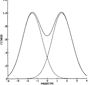
Figure 1 shows the relationship between fitness and phenotype that will be assumed throughout this paper. The fitness curve is the sum of two Gaussian curves, each characterized by its height, by the position of its peak, and by its standard deviation. Gaussian (normal) curves are chosen here both for their mathematical tractability and for their biological reasonableness. Selection of this sort, when directed against departures from a single optimum phenotype, is usu-

PHENOTYPE

NATURAL SELECTION FOR TWO OPTIMA 775

ally called “nor-optimal’’ selection. Several symmetry assumptions will be made throughout this paper. The two Gaussian components will be assumed to be of equal height and to have equal width (as expressed by their “fitness variance”

S). Their peaks will be assumed to be at P and -P, so that the fitness curve is centered at the origin. This last assumption is not restrictive, as the origin of the phenotype scale is in any case arbitary.

The fitness function is then

w ( X ) = exp[-1/2 (X-P)2/S]

+

exp[-l/2 (X+P)2/S]

.

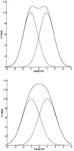
(1) When S

<

P2, this curve is bimodal, the two peaks of w ( X ) lying respectively between P and 0 and between -P and 0. When S 2 P2, the curve is unimodal, with peak at zero. These facts are illustrated in Figure 2. Note also that the func- tion (1 ) is scaled so that each component has height unity. Since we shall be con- cerned only with relative fitnesses and never with absolute fitnesses, this arbitrary choice presents no problems.

We shall frequently make use of a simple property of (1), which is worth noting. Natural selection in which each individual is exposed to selection accord- ing to the fitness function w(X) will have the same results as selection in which half of the individuals (chosen randomly with respect to phenotype) are exposed to nor-optimal selection with optimum phenotype P , and the other half exposed to nor-optimal selection with optimum phenotype -P. This follows from the sim- ple fact that if f ( X ) is the density function of the distribution of the phenotype X in the population before selection acts, after it acts the density is proportional to f ( X ) [wl(X)

+

w2(X)], which must of course be equal to f ( X ) wl(X)

+

f ( X ) wz (X)

.

This latter (disregarding a constant multiplier) is also clearly the density function of X among survivors of selection when selection for the two optima P and -P act on different individuals. I n the above expressions, w,(X) and w2(X) refer to the two terms of (1). This must be distinguished from the case in which we take the survivors of the two sorts of selection and mix them in predetermined proportions. I n that case, which we do not consider here, the den- sity function of mixed survivors would be proportional to f ( X ) wl(X)

J

El

4-

f ( X > wz(X)

/

Z2. The present model is equivalent to mixing the two groups of survivors with the frequencies of the two groups in the resulting mixture being proportional to

W l

and W z .

T H E GENETICS O F T H E PHENOTYPE

We assume an outbreeding, random mating, diploid organism with discrete generations and a n infinite population. The phenotype X is determined by n loci. There is assumed to be additivity of allele effects, not only between loci but also within loci. Thus there is not only no epistasis, but also no dominance i n the determination of this phenotype.

776 JOSEPH FELSENSTEIN

1.2r

PHENOTYPE

1.4-

1.2-

1.0-

(0

a -

9

v)

c LL

w *6

-

.4

-

PHENOTYPE

FIGURE %-The transition between bimodality and unimodality. In both cases P = 1. Figure

NATURAL SELECTION FOR TWO O P T I M A 777

phenotype.

A

genotype may be represented by a 2n-tuple ( x l , x2,

. . . ,

Xn,Xn+1,

. . .

xzn) where xi is the contribution of ith gene copy to the phenotype, so that

We shall follow the convention that x l ,

. . .,

x n are the maternally derived alleles at loci 1,

.

.

.

,

n and x ~ + ~ ,

.

. . ,

x z n the paternally derived alleles. The major ap- proximation we will make is to assume that in any generation, the genotype vectors x follow a multivariate normal distribution. This approximation was in- troduced by LANDE (1975), and I have discussed it in some detail elsewhere

(FELSENSTEIN

1977). I n the case of simple nor-optimal selection, multivariate normality is exact essentially only when there is no recombination (FELSENSTEIN 1977), but it is nevertheless a most useful approximation. I t avoids the computa- tion of higher-order linkage disequilibria, since the multivariate normal distribu- tion is completely described by the means, variances and covariances of the 2n variables.

In the present case, the assumption of multivariate normality is expected to be less satisfactory than in the case of nor-optimal selection. As we shall see in the exact numerical analysis of a ten-locus model below, when recombination is tight the phenotype distribution can become strongly bimodal. Without the assumption of multivariate normality, I have been unable to obtain any analytic results. As

shown later by the comparison of the analytic results with exact numerical itera- tion of multi-locus models, as well as with analytic treatment of a two-locus model, the results obtained do not appear to be very sensitive to this assumption. Note that the model implicitly assumes, in using the multivariate normal approxi- mation, that there is an infinite number of alleles at each locus, with a normal distribution of !heir phenotypic effects xi.

We shall restrict the genetic model by further assuming that immediately after random mating the means, variances, and covariances are equal at all loci:

E ( x i ) = m

i =

1 , 2 , .

.

.

, 2 n (3a) E [ ( ~ i - m ) ~ ] = U

i =

1 , 2 , .

.

.

,2n (3b)

E [ ( x i - m ) ( s j - m ) ] = c

i

= 1 , 2 , .

.

.

,

n, (3c)

i = 1 , 2

, . . . ,

n,

i

#

j .

This assumption of exchangeability of loci can be sustained only at the cost of a further assumption about the genetic system: that the recombination fractions between all pairs of loci are equal, so that r,j = r . This does not correspond to a realizable genetic map unless r = 0 or I = 0.5. With all of these approximations, our model now resembles the models of SLATKIN (1970) and BULMER (1971), with the exception that we have an explicit finite number of loci n. Note that the

state of the population can be represented in this approximation by only three quantities: M = 2nm, V = 2nv, and C = 2n (n-1) c. For a population immedi- ately after random mating, these represent the phenotypic mean ( M )

,

that part

778 J O S E P H FELSENSTEIN

due to linkage disequilibrium ( C ) . The total phenotypic variance is V

+

C. By following the changes in M , V , and C , the effects of mixed disruptive and stabi- lizing selection will be investigated. I n particular, a simple rule with nontrivial consequences will be found that predicts whether natural selection will result in a “specialist” or a “generalist” phenotype. As we shall see, a limited verification of this rule in two-locus, two-allele models is available, and indicates that the rule may generalize to many different genetic situations. For the moment we defer consideration of the accuracy of our multivariate normal approximation and our exchangeability assumptions. This difficult question will be dealt with in a limited way when we discuss the results of four-locus, two-allele numerical iterations.

THE EQUATIONS O F C H A N G E

APPENDIX 2 outlines the derivation from LANDE’S equations of the recurrence relations for change in M , V and C under nor-optimal selection with a single peak. In our model, the life cycle is assumed to be:

Adults -

-+

Zygotes--- > Adults

With selection for two optima being equivalent to selection of half the population for each optimum, followed by mixture of the survivors, this must be equivalent to:

random mating selection

random mating selection mixture

Adults

---+

Zygotes ----A Adults __- Adults

Random mating of diploid individuals is equivalent to random union of their gametes, so that we might as well deal with the model in which the survivors of

selection produce gametes, and these then mix in the appropriate proportions and unite at random to produce the zygotes of the next generation:

Gametes

-

Zygotes -4 Adults Gametes

+

Gametes

APPENDIX 2 tells us that if the survivors of selection for one optimum were to produce zygotes by random union of gametes, the observed changes in M , V and C would be:

random combination selection recombination mixture

M * =

(s+

V t C

I +

1

(v+c>2

v* =v--

2n

s+v+c

(s+v+c

v+c

I

where

P

is the optimum phenotype in the particular component of the fitness curve that exerts this selection.

NATURAL SELECTION FOR TWO OPTIMA 779

would find if the gametes produced by the survivors of selection for optimum phenotype

P

were allowed to combine at random. APPENDIX 2 demonstrates that when gametes mix from two gamete pools characterized respectively by

Mi*,

Vi*,

Cl*

and M 2 * , V,*, C,* i n proportions pi and p 2 , and then allow them to unite at random, the resulting population of zygotes has

NI'= p l

Mi*

+

p z M2*

,

1

2n

V' = pi Vi*

+

p2 V2*

+

-pi pz

(Mi*

-

Mz*)'

,

(5c)

1 1

c'

= p i

Cl*

4-

p2 C2*

4-

- 2 (1 -

-)

n p i p z (Mi*

-

M 2 * ) 2

.

In APPENDIX 2, it is shown that among those individuals exposed to selection with optimum phenotype

P,

the proportion of survivors will be

1

S 1

(M-P)'

with a similar expression for E, when the optimum phenotype is

-P.

The fraction of all survivors who come from subpopulation 1 is then

which gives, using equation (6) and its analogue,

and where

We are now in a position to substitute equations (8) and

(4)

into ( 5 ) , obtaining as our basic recurrence relations:

S D-1

(9b) 1 (V,+Ct)'

+-

1 4 0

(vt+ct)z~p27

Vt+l = Vt --

2n (S+Vt+Ct) 2n (l+D)2 (S+Vt+Ct) and

780 JOSEPH FELSENSTEIN

equations, but we shall see that some information can be gleaned from them ana- lytically, and some from computer iteration, to yield rules for the outcome of bimodal selection.

EQUILIBRIA O F T H E SYSTEM

We will examine the outcome of selection for two optima by finding the equilibria of the recursion (9), and by partially characterizing the stability of those equilibria, in the hope that the system does not have any limit cycles. At various points, it will be necessary to appeal to the experience of numerical iteration of this system to complete its analysis.

First, let us use (9b) and (9c) to produce the recursion relation for the quantity (n-1) V t

-

Ct. When this is done, there is a great cancellation of terms, resulting in

(10) Setting

Vt+l

=

V t

and

Ct+l

= C t , this becomes simply Ct r = 0. Thus, at equi- librium we must have either r = 0 or

C

= 0, or both. For the moment, assume that C = 0. Examination of (9b) shows that if

V t + l

= V t and Ct = 0, then for any finite S and any finite n, we must have either

( n

-

1) Vt+1- Ct+1= ( n

-

1) vt -

ct

+

Ct r

.

v=o

or

4D P 2 - s . (l+D)’

V =

Of course, the latter is not an explicit solution for

V

in terms of the other quanti- ties since we can see from equation (8c) that D contains

V

and

M .

If we assume that the condition that holds at equilibrium is (1 l a ) , then (9a) shows us the interesting property that any value of

M

is an equilibrium value! If, on the other hand, ( 1 1 b) holds, then since P2

>

0 we must have that

M = ( - )

D-1 P . D+l

But from (8c) and (1 lb)

D = exp

[ M

( 1 + D ) 2 / ( 2 P D ) ]

.

(13) Both (12) and (13) must hold if (1 l b ) does and there is equilibrium. So, we can solve both ( 1 2 ) and (13) for M / P , and equate the two resulting expressions, which are functions of D, obtaining finally

D 2 - 1 2 0

--

- - In D

When D = 1, condition (14) is satisfied. There is no other point of intersection of the two sides of (14) for D

>

0. When

D

= 1 , since P

>

0, we must by ( 8 ~ ) have M = 0. Then from (1 lb)

NATURAL SELECTION FOR T W O OPTIMA 781

The case when I = 0 is of less interest, simp there will frequently be serious

violation of multivariate normality in that case. One can add (9b) and (Sc), in this case, to obtain two-variable recurrence equations in

Mt

and Vt

+

Ct. The equilibria turn out to be

v+c=o

M = O

and V + C = P 2 - S .

o r , i f P 2 > S ,

Thus, putting all of this together, the conditions for equilibrium of the recur- sion (9) reduce to (16) and (17), with the further stipulation that, if r

>

0,

then C = 0 at equilibrium.

STABILITY O F T H E EQUILIBRIA

We have now found two classes of equilibria.

If

we represent the state of the system by the point

( M ,

V , C), and consider only the case in which I

>

0, we

can represent these two classes of equilibria by the line

( M ,

0,O) and the single point (0, P2

-

S, 0). We will need an analysis of the stability of these equilibria to indicate toward which of these values the system is likely to move.

In

addition to concerns about normality, a major limitation of the kind of stability analysis we carry out here is that it stays within the framework of our exchangeability assumptions. We will consider the effects of perturbing the quantities M ,

V

and

C from their equilibrium values, but we are unable to consider the effects of asymmetries. We always assume that all individual locus variances and all covariances between loci remain equal throughout the dynamics of the system. The two- and four-locus models to be presented below are in part an attempt to check the adequacy of the exchangeability assumption.

First, let us consider the line of values

( M ,

0,O). Any point in this line is an equilibrium, corresponding to our intuitive expectation that, when there is no

genetic variation

(V

= C = V+C = 0), there can be no genetic change. Now

suppose that we perturb the system from one of these equilibria to the point

( M

+

x,

y , z )

.

We can use (9a)

-

(9c) to obtain expressions for

x',

y' and

z',

the values of these perturbations in the succeeding generation. When in those expres- sions all terms of order x2, y 2 , z2, zy, y z and

xz

are ignored, we obtain the first- order approximation

and

Y ' " Y ,

2

' z(1-r)

.

It should be clear that this linearization cannot show local stability of the equilibrium, for in it, as in the full system, any perturbation to the point

( M

+

x,

782 JOSEPH FELSENSTEIN

of quadratic terms would be necessary to determine the behavior of the system when perturbed from one of the points on the equilibrium line. However, if the point

( M ,

0,O) is found to be locally unstable, then it is known that it must also be asymptotically unstable (when all terms are taken into account). In fact, the latter is usually the case. The approximate recursion system shows neutral stability in y. Perturbations in this variable simply remain, neither growing nor declining to zero. I n variable

x,

this implies that, since z declines to zero and y

remains constant,

x

will change at a constant rate in a direction depending on y but not on x. This means that the system will be unstable in the variable z unless the coefficient of y is zero, so that

--+(-)

M D--1 P - 0 .

S D + l

s-

It is not simple to solve this for M , since D is a function of M , given by (8c). Substituting (8c) into (1 9) and solving for

M / P ,

we obtain

This equation is satisfied when M = 0. When

P2

>

S, it also has two other roots, symmetrically placed, at

M

= f

P*.

After some tedious algebra, one may verify that the points P* at which (20) is satisfied are precisely the maxima of the

function

w(X)

given by (1). This argument has identified points at which the local stability analysis does not predict instability. At these points, the system cannot show asymptotic stability in the strict sense, since if it is perturbed from them to another point on the line ( M , 0,O)

,

it will not return. These points can at best show asymptotic stability only in the sense that the system will return to them if perturbed to any nearby point not on the line

( M ,

0,O).

W e have now found four equilibrium points of the system that have a chance to be stable when r

>

0:

(i) M = V = C = O ,

(ii) M = 0, V =

P2

- S, C = 0 (iii) and (iv)

M

= f P*, V = C = 0

(provided

P2

>

S)

(provided

P2

>

S )

When r = 0, we can do much the same analysis in two variables, with V+C in place of V . The results are essentially identical.

Equilibria (i), (iii) and (iv) are easily given an intuitive interpretation. In

NATURAL SELECTION FOR TWO OPTIMA 783

on the slope of

w ( X )

locally, as it depends on the fitnesses of the restricted range

of phenotypes that actually occur in the population. Since M responds to selec- tion on a much faster scale than

V ,

the population mean will be expected to move in the direction of increasing w ( M ) and to complete this motion long before

V

and C disappear. Thus, we expect the population mean ultimately to arrive at a peak of the fitness function and stay there. When P2 5 S, there is only one peak, at

M

= 0. When P 2

>

S, there are two peaks, at

M

= P* and

M

= -P*. Thus, we expect equilibria (iii) and (iv) to be stable whenever they exist, and equi- librium (i) to be stable whenever (iii) and (iv) do not exist.

These are only expectations, based on a crude intuitive argument. The full analysis of the stability of these equilibria would require consideration of the higher-order terms that have been dropped from (18a-c)

,

to say nothing of what would be involved in analysis of the global stability regions of these equilibria. Rather than attempt such an analysis, I will rely only on the experience of

iterating the recursion (9) numerically. This has, in every case run, confirmed the above intuitive arguments and showed convergence to a peak of the fitness function, with ultimate elimination of genetic variation. Furthermore, when the two equilibria (iii) and (iv) exist, which of them the population finally approaches is determined by the initial sign of

M .

That this is to be expected may be seen from (9a). That equation shows

Mt+l

to be a weighted average of the quantities M t and ( D - l ) / P ( D + l ) . A consideration of (8c) will show that this quantity will have the same sign as M t . Thus will have the same sign as M t .

This would make a rather neat picture were it not for the rather mysterious equilibrium (ii). When we attempt a linear analysis of the stability of this equilibrium by letting

M

=

x,

V = P2---S+y and C = z , we find after dis- carding terms in x2, y 2 , 2, xy, y z and

xz

that

x

'

5

z ' " z ( 1 - r ) - ( y + z ) [ T ( l 1

--)

1 _{( 1}

_{- F )}

_{s 2}

1.

n

784 J O S E P H FELSENSTEIN

species analysis of character displacement by SLATKIN (1979a)

,

who also used normal approximation techniques.

With the elimination of (ii) as a final autcome, we have a relative simple rule in which the outcome of evolution depends only on whether P 2

>

S and possibly on the initial sign of

M .

P A R T I A L HERITABILITY O F THE CHARACTER

The simplicity of the results in previous sections corresponds to the simplicity of the model. The phenotype has been assumed to be the sum of contributions of individual allele effects. This has not allowed for any environmental effects on the character. A more biologically relevant model would incorporate a random environmental effect e. which is added to the sum of gene contributions:

Y = X + e

(22a>

For simplicity we take e to be normally distributed with mean zero and variance

E , and independent of all of the xi. The phenotype is now given by

Y .

The quan- tity X is the breeding value (or additive value) of the genotype. The fitness function will be given by (1) with Y in place of X .

We may inquire how fitness depends on the breeding value X . For selection for a single optimum, it is known (LANDE 1975; FELSENSTEIN 1977, p. 238) that fitness as a function of breeding value is, in our present notation:

(23 ) 1

2

w ( X ) = (1

+

E / S ) - 1 / 2 exp [-

-

( X

-

P ) 2 / ( S

+

E ) ]

.

Except for the multiplicative constant in front, this is of the same form as the first term of ( l ) , provided that S is replaced by S

f

E . Now the fitness of a given breeding value X under bimodal selection will be the sum of two terms, each of € o m ( 2 3 ) , in direct analogy to (1). The fitness function

w ( X )

will thus be of the same form as ( l ) , except for the constant factor (1

4-

E / S ) - 1 / 2 and the replacement of S by S -t E , T h e constant factor has no effect on the dynamics or the outcome of selection, which depends only on the relative fit- nesses, not on the absolute fitness. Furthermore the interpretation of X as a phenotype rather than a breeding value did not enter into our previous argument in an essential way.

Thus, we can use the results of the previous sections in the case of partial heritability, provided only that we reinterpret X as being the breeding value and w ( X ) as the curve of fitness as a function of breeding value, and replace

S by S -I- E throughout the argument. The results are straightforward: whenever

P'

>

Sf

E , we expect the population mean to arrive ultimately at the peak of

NATURAL SELECTION FOR TWO OPTIMA

785

near-trival result: that whether the population will become generalized o r spe- cialized depends on whether the fitness function is unimodal or biomodal. But

this trivality is only on the surface-this simple rule has surprising consequences. Recall that w ( X ) now gives fitness, not as a function of phenotype, but as a function of breeding value. The conditions for bimodality or unimodality of

w

( X ) differ from those for bimodality o r unimodality of the curve giving fitness as a function of phenotype. Comparing ( 2 3 ) with the first term on the right hand side of (1) shows that the presence of environmental variance in the phenotype fattens the individual components of w ( X )

,

increasing the standard deviation of an individual peak from S1I2 to ( S

4-

E ) 1 / 2 . When S

<

P2

I

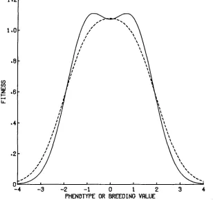
S

f

E, the breeding value fitness curve will be unimodal even though the phenotype fitness curve is bimodal. Figure 3 shows these two curves plotted for such a case. For a given regime of selection for two optima, we can conclude that the population is less likely to respond by becoming generalized in phenotype, the less environmental variance there is in the phenotype. Thus the lower the initial heritability of the character, the more readily it will respond to selection by arriving at a generalized phenotype. We may also note that as the individual

1.2.-

1.0-

.0

-

(D (D

w

z . 6 -

t;

LL

.4

-

1

-4 -3 -2 -1 0 1 2 3 4

PHENOTYPE

OR

BREEDING

VALUE

786 JOSEPH FELSENSTEIN

component peaks of the fitness function are widened, not only does the function become more unimodal, but the positions of the peaks P* and

-P*

move toward zero. Although there is a sudden transition from bimodality to unimodality as

S

4-

E reaches P2, this is accompanied by a continuous approach of P f and

-P*

to zero, where they collide when

P2

= S f E . A further consequence of low heritability (large E ) is that it displaces the equilibrium specialized phenotypes towards each other. Thus, we should expect not only a lower probability of occurrence of specialization in a low-heritability trait, but also a less complete specialization.

These results are similar to those of LEVINS (1962), who identified (S

f

E ) - l l 2 as a measure of homeostasis, in that it measured how rapidly fitness fell off as the phenotype deviated from its optimum value. The present results are consis- lent with his prediction that specialization would be more likely the larger the niche difference was compared to the tolerance for environmental diversity. I n the present terms, this amounts to a comparison of P with (S -I- E)lI2. The cur- rent results make LEVINS’S (1962) predictions more specific by providing a more detailed genetic model and a particular fitness function.

All of the above results have assumed that the fitness curve is symmetric, the two modes having equal height. However, the results are not sensitive to this assumption. With asymmetry of the fitness curve, the condition for selection to favor specialization will still be that the curve relating fitness to breeding value be bimodal. This asymmetry does make the conditions for existence of this bimodality more restrictive. A larger value of

P

(or a smaller value of S -t E ) will be required to have bimodality if the modes are of unequal height.

EXACT RESULTS WITH TWO-ALLELE MODELS: FOUR-LOCUS A N D TEN-LOCUS ITERATIONS

These remarks having been made, there must still remain some nagging doubts about the results. We have employed an approximation, and have found that the stability of equilibria is surprisingly delicate, involving higher-order terms. Surely we are justified in being skeptical of the robustness of the results. This concern will be addressed here in two rather limited ways. The first involves numerical iterations. Exact deterministic numerical iterations have been carried out with a four-locus, two-allele model subjected to selection for two phenotypic optima. The allele effects at the four loci were taken to be equal to

k0.5, so that the possible breeding values of the genotypes range over all integers from

-4

to

4.

The phenotypes for each genotype were assumed to be normally distributed around its breeding value, with variance E . Natural selection on phenotypes was given by (1). Under these circumstances, the fitnesses of the genotypes are readily calculated, and it is straightforward to carry out iteration of gamete frequencies from generation to generation.

NATURAL SELECTION FOR T W O OPTIMA 787 value of S

+

E

is 3: which is less than P? =

4.

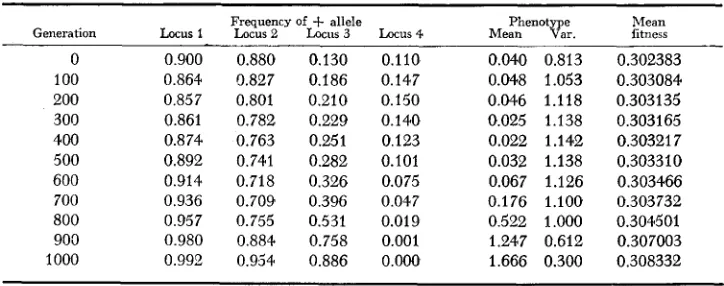
The population is started in linkage equilibrium near a position of mixed fixation in which two loci are fixed for the +allele and two for the -allele. In every case, the results of the four-locus simulation have conformed to the results expected from the multivariate normal approximation. I n the case of Table 1, after spending many generations near

M = 0 and with phenotypic variance near 22 - 3 = 1, that state ultimately proves unstable, and the population proceeds toward fixation for

-

alleles at three loci and

4-

alleles at one, so that M = 2 with no genetic variance at equilibrium.

To what extent may we regard these numerical iterations as verifying the accuracy of our previous approximations? The results of previous sections were based on normality and exchangeability assumptions imposed on an n-locus model having a continuum of alleles at each locus. W e may regard the four- locus, two-allele results as a different way of approximating to this model. These two approximations yield results consistent with each other. Alternatively, we may regard the n-locus, infinite-alleles model as itself being a n approximation to an n-locus, two-allele model. Whichever approach we take, the congruence of results indicates that there exists some larger class of models for which our present results hold. The four-locus, two-allele results indicate that the validity of our rules for the outcome of selection is not critically dependent on either the maintenance of multivariate normality or the maintenance of exchangeability of

loci.

The experience of numerical iteration does indicate that multivariate nor- mality is likely to be a poor approximation when linkage is tight. When there is no recombination, it is a simple matter to carry out numerical iteration of

a

model with ten loci and two alleles per locus, for if the loci have equal effects and show no dominance, the equations are the same as those for an eleven-allele,

TABLE 3

Results of 1000-generation iteration of a four-locus, two-allele model with additive effects of equal size at all loci

~ ~

Mean Generation Locus 1 Frequency of Locus2 Locus -k allele 3 Locus4 Me:?OtKr. fitness 0 0.900 0.880 0.130 0.110 0.040 0.813 0.302383 100 0.864 0.827 0.186 0.147 0.048 1.053 0.303084 200 0.857 0.801 0.210 0.150 0.046 1.118 0.303135 300 0.861 0.782 0.229 0.140 0.025 1.138 0.303165 400 0.874 0.763 0.251 0.123 0.022 1 .I42 0.30321 7 500 0.892 0.741 0.282 0.101 0.032 1.138 0.303310 600 0.914 0.718 0.326 0.075 0.067 1.126 0.303466 700 0.936 0.709 0.396 0.047 0.176 1.100 0.303732 800 0.957 0.755 0.531 0.019 0.522 1.000 0.304501 900 0.980 0.884 0.758 0.001 1.247 0.612 0.307003 1000 0.992 0.954 0.886 O.OO0 1.666 0.300 0.308332

788 JOSEPH FELSENSTEIN

one-locus model. Numerical iteration of such a model is quite inexpensive. It

shows that when the fitness curve is strongly bimodal, and when the population mean M is near zero initially, the distribution of breeding values of gametes can become strongly bimodal. While the distribution of breeding values of gametes remains unimodal in the case of Table 1 , where r = 0.1, it would have become bimodal if linkage had becn much tighter.

For all of these indications of departure from multivariate normality when linkage is tight, the ten-locus, two-allele model without recombination continues to follow our rules for the outcome of selection. Specialization is the ultimate outcome when the curve of fitness uersws breeding value is bimodal, generaliza- tion when it is unimodal. This is further indication that the validity of these rules goes far beyond the set of models for which normality and exchangeability are good approximations. These numerical iterations provide very weak verifica- tion of the accuracy of the multivariate normal model and of the generality of its results. However, they will have to do until someone ilinds a better way to verify the accuracy of these approximations. It is an unfortunate fact that we cannot make use of weak-selection perturbation approximations for this purpose. With weak selection, the fitness curve is necessarily u n i m d a l , and there would be no way of investigating the effects of bimodal selection using such a n approach. There are actually two sorts of exceptions to the rule that the results of the four-locus and ten-locus iterations were the same as those of the normal approxi- mation. The first is that the condition for convergence to the central equilibrium was not P2 5 S

+

E , but was unimodality in the plot of fitness against breeding value. When there are a finite number of possible breeding values, as in any model with a finite number of alleles at a finite number of loci, the conditions

for unimodality become slightly weaker than

P2

5 S

f

E. We consider this mat- ter further in the last section of this paper.

The second exception to the patterns seen in the normal approximation is that when the fitness curve is bimodal, and when the genotype of highest fitness is not homozygous at all loci, there can be a small amount of heterozygosity main- tained at equilibrium; not all genetic variance disappears. The expense of the four-locus iterations made it difficult to investigate the nature of these equilibria. I n the next section, we consider a two-locus model in which some of these ques- tions can be addressed analytically.

ANALYTIC RESULTS FOR A TWO-LOCUS MODEL

The second check of our approximations involves a two-locus model. If we have a two-locus, two-allele model in which the phenotype is the sum of allele effects, in which the allele effects are the same at the two loci, and in which the two cptimum phenotypes happen to be symmetrically distributed around the inter- mediate phenotype, the table of htnesses will have the form:

BIB, _{-.___._} BIB,

4%

A I A I b a 1

A A a 1 a

NATURAL SELECTION FOR T W O OPTIMA 789 This is a special case of the general symmetric model of

BODMER

( BODMER and PARSONS 1962; BODMER and FELSENSTEIN 1967). The general symmetric model was analyzed rigorously in many aspects by KARLIN and FELDMAN (1970). I n their terms, the present model has (Y = 0, ,B = y = l-a, and 6 = l-b. Unfor-

tunately, their results are inapplicable to the present case, as they largely restricted their attention to cases in which a

>

0.

The bimodal Gaussian fitness function ( 1 ) places restrictions on the values of a and b. In particular, it implies that when a

<

1 , b

<

a*, and when a

>

1 ,

b

<

d ( 2 c z - 1 ) . However, we shall consider all positive a and b, with the excep-

tion that we do not allow the case b

>

a

<

1 , as that would imply three peaks in a plot of fitness against breeding value. There are three cases we will want to distinguish:

(i) b

<

a

<

1.

I n this case, the fitness function is unimodal when plotted

against the breeding value.

(ii) b

<

a

>

1 . The fitness function has two peaks, which occur at genotypes heterozygous at one locus.

(iii) b

>

a

>

1.

The fitness function has two peaks, which occur a t doubly homozygous genotypes.

We will not concern ourselves with cases of exact equality of any of the three quantities a, b, and

1,

as these are of little biological interest.

Equilibria with fixation at both loci

There are four equilibria that are fixed at both loci. The two equilibria fixed for the extreme genotypes A,A,B,E, or A,A,B,B, are both stable in our case (iii)

,

but are unstable in cases (i) and (ii)

.

Thus, they are stable only when the genotype that is fixed is the one with highest fitness. The other two equilibria fixed at both loci are fixed for the genotypes A,A,B,B, and A,A,B,B,. These turn out to be stable in case (i) but not in cases (ii) and (ii) and (iii). Again, stability obtains only when the corresponding genotype is the one with the highest fitness. These conclusions are easily obtained from the conditions given by BODMER and FELSENSTEIN (1967 j

.

Equilibria with fixation at one locus

There are clearly four such equilibria, depending on which allele at which locus is fixed. Since a necessary condition for stability of such an equilibrium is overdominance a t the segregating locus, only in case (ii) it is possible for these equilibria to be stable. Carrying out the necessary algebra, one finds that the conditions given by BODMER and FELSENSTEIN (1967, Table

5)

predict that such an equilibrium exists and is stable if and only if a

>

b

>

1. This is the subcase of (ii) in which the intermediate phenotype has the lowest fitness of all. Equilibria with both loci segregating

(I) Symmetric equilibria: KARLIN and FELDMAN (1970) has shown that in the general symmetric model there is always at least one equilibrium having

790 J O S E P H FELSENSTEIN

equilibria for a sufficiently small recombination fraction. Otherwise, there is one symmetric equilibrium. Computation of the critical threshold value of the recom- bination fraction involves solution of a cubic equation, which will not be at- iempted here.

Unfortunately, the conditions f o r stability of these symmetric equilibria given by KARLIN and FELDMAN (1970) cannot be used in the present case, as they restrict their attention to the cases in which CY

>

0. The conditions given by

BODMER and FELSENSTEIN (1967) are difficult to apply, as they state that limits on r are given by the solution to a cubic equation whose coefficients depend on r, as noted by KARLIN and FELDMAN (1970). When selection coefficients are weak, these conditions could be evaluated approximately, but we are interested in both strong and weak selection.

We will not attempt a n algebraic derivation of conditions for the stability of these equilibria, but instead will rely on experience with numerical iteration of the gamete frequencies. Examination of many different values of a, b and r indicates that symmetric equilibria are stable only in case (i), when

a

<

(1

4-

b ) /2, and then only for small 1. The particular equilibrium involved

has an excess of the coupling gametes A,B, and A&.

It

should be noted that if the values of a and b are generated by mixture of two normal distributions as given by (I), in case (i) we can only have a

<

(1

+

b ) /2 if a

<

0.543689, which is rather strong selection.

Thus, a stable symmetric equilibrium seems to exist only in some cases with strong selection and unimodal fitness curve, and then only for restricted recombination.

(11) Nomymmetric equilibria: KARLIN and FELDMAN (1970) discovered a class of nonsymmetric equilibria, of which as many as four could exist at once.

They gave existence and stability conditions for them when CY

>

0. I n the present

case, in which a = 0, it is not difficult to verify that two nonsymmetric equilibria

of the form

exist, where two values of p can be obtained by solving for p in

This is a pair of equilibria having the property that P ( A , ) = P ( B , ) with no linkage disequilibrium. It is readily shown that the equilibria (24) have positive frequencies for all gametes only if (a-1) (b-1)

<

0. Among OUT cases, only the subcase of (ii) having b

<

1 satisfies this condition. This is precisely the case in which the equilibria fixed at one locus are unstable.

NATURAL SELECTION FOR T W O OPTIMA 791 condition for equilibria having

D

= 0 given by

BODMER

and

FELSENSTEIN

(1967) fails to find any range of values of r for which instability is predicted.

A

general method for locating equilibria in multiple-locus models with sym- metry constraints has been developed by SLATKIN (1979b). He finds (SLATKIN, personal communication) for the present model that one class of equilibria whose existence it permits is that in which P ( A , B , ) = P ( A , B , ) . The present nonsym- metric equilibria fall within this class.

Summary of equilibria

The stable equilibria we have found can be summarized as follows.

(i) b

<

a

<

1. Fixation for either of the gametes A,B, or A,B, is stable. For a

sufficiently small recombination fraction, there is a stable polymorphism with all alleles equally frequent and an excess of coupling gametes, provided that a

<

( l + b ) / 2 .

(ii) b

<

a

>

1.

If

b

<

1, there are two stable, nonsymmetric equilibria having no linkage disequilibrium, with P ( A , ) = P ( B , )

.

If

b

>

1, there are four stable equilibria, which segregate at one locus and are fixed at the other.

(iii) b

>

a

>

1. Fixation for either of the gametes A,& or

A&

is stable. The general picture we derive from the two-locus analysis is that when the genotype with the highest breeding value (the highest genotypic mean fitness) is a double homozygote, the population will fix for that genotype. When the genotype with the highest fitness is a single heterozygote, polymorphism at one or two loci will be maintained, depending on the exact fitness pattern. The only feature of the two-locus model inconsistent with the conclusions from the normal approximation is the existence of a two-locus polymorphism with strong coupling disequilibrium when fitnesses are unimodal. However, this requires both strong selection and tight linkage.

EFFECTS O F T H E DISCRETENESS O F GENOTYPES

Our results for two loci have validated the distinction between bimodality and unimodality of the selection curve. When the central genotype is no longer the one with highest fitness, fixation for it becomes unstable. This is, of course, a

slightly different criterion from unimodality of the continuous curve of fitness as a function of breeding values. We now briefly inquire whether this is likely to have a strong effect on the results.

Suppose that we have a fitness function with two components, placed at P and -P, each with variance

H E .

The condition for the resulting fitness function to be bimodal is clearly P2

>

S+E. Now, suppose that we evaluate the function at a discrete grid of points, corresponding to different genotypic mean pheno- types, such that the peak P is n points away from the center 0. Then, we can observe bimodality only if the height of the curve at P / n exceeds its height at 0.

792 J O S E P H F E L S E N S T E I N

Letting y = e x p

[-l

2 1

,

the point at which the two sides of (25)

2 S + E

become precisely equal becomes

Y ( l - l / n P

+

y ( l + l / n ) * = 2 Y . ₍₂₆

₁

For any given value of n, this can be solved for

y

by numerical methods. Using

-

2 In y =

P z / ( S

+

E ) ,

we find:

n P / ( S + E ) 1 / 2 for bimodality

1 2 3 4 5 10 20

00

1.10397 1.021898 1.0094~6 1.00527 1.00336 1.00083 1.00021 1 .o

While there is a slightly more stringent requirement for bimodality when the

number of genotypic classes is small, this rapidly disappears

with

more geno- types. Although the discreteness of genotypes makes phenotypic specialization slightly more difficult, clearly we will err very little by assuming that bimodality

of the continuous curve giving fitness as a function of breeding value is the con- dition for natural selection to favor development of a specialized phenotype. The effects of assuming an infinite number of loci must be far smaller than the effects of the many other special assumptions made in the present model.

I thank TOM NAGYLAKI, RUSSELL LANDE, MONTY SLATKIN, MICHAEL BULMER, PETER AVERY, MASATOSHI NEI, SAMUEL KARLIN and a referee for helpful comments. This work was supported by US. Department of Energy contract number EY-76-S-06-2225 #5 with the University of Washington.

LITERATURE CITED

BODMER, W. F. and P. A. PARSONS, 1962 Linkage and recombination in evolution. Advan. Genet. 11: 1-100.

BODMER, W. F. and J. FELSENSTEIN, 1967 Linkage and selection: theoretical analysis of the deterministic two-locus random mating model. Genetics 57 : 237-265.

BULMER, M. G., 1971 The effect of selection on genetic variability. Am. Naturalist 105:

201-211.

DICKINSON, H. and J. ANTONOVICS, 1972 The effects of simultaneous disruptive and stabilizing selection. Heredity 29: 363-365.

NATURAL SELECTION FOR T W O OPTIMA

793

KARLIN, S . and M. W. FELDMAN, 1970 Linkage and selection: two-locus symmetric viability model. Theoret. Pop. Biol. 1: 39-71.

LANDE, R., 1975 The maintenance of genetic variability of mutation in a polygenic character. Genet. Res. 26: 221-235.

LEVINS, R., 1962 Theory of fitness in a heterogeneous environment. I. The fitness set and adaptive function. Am. Naturalist 96: 361-373.

MATHER, K., 1955 Polymorphism as an outcome of disruptive selection. Evolution 9: 52-61.

MAYNARD SMITH, J., 1962 Disruptive selection, polymorphism and sympatric speciation. Nature

SLATKIW, M., 1970 Selection and polygenic characters. Proc. Nat. Acad. Sci. U.S. 66: 87-93. SLATKIN, M., 1979a Ecological character displacement. Ecology (in press). -, 19791, A

note on the symmetry constraints imposed by dominance in multiple locus genetic models. Genet. Res. 33: 81-88.

Corresponding editor: M. NEI

195: 60-62.

APPENDIX i

Multiplication and inuersion of certain patterned matrices

Let I be the usual 2n

x

2n identity matrix, which has ones down the diagonal and zeros

off the diagonal. Suppose that U is the n

x

n matrix whose elements are all one. Then we define two 2n

x

272 matrices, J and K, as

and

( A l - I )

(Al-2)

so that K is the 2n x 2n matrix of ones. The following rules for multiplication of these matrices are easily derived:

U

= J I = J,

IK = KI = K, J z = nJ,

Kz = 2n K,

J K = K J = nK.

and

(Al-3) (Al-5) (AI-6) (A1-4.)

(Al-7) Using these relations, we can readily compute the product of any two matrices that are of the form a1

+

bJ

+

cK. By setting up two such matrices, taking their product and requiring the result to be 11

+

OJ

+

OK, we can equate terms i n I, J, and K, and on solving for the coefficients of one matrix in terms of the other, we obtain the matrix inversion rule:

K , (AI-8)

1 b

a a ( a + n b ) ( a

+

nb) ( a

+

nb

+

2nc)

( a I + b J + c K ) - 1 = - 1 , - - -

J--L---

which will hold whenever the inverse exists.

A P P E N D I X 2

EfJect of selection for a single-optimum phenotype

equations ( 2 ) and ( 3 ) . Assume the single-optimum fitness function

Assume the multivariate normal approximation with exchangeability of loci, defined in

(A2-1) 1

2

794 JOSEPH FELSENSTEIN

The following results were first obtained by LANDE (1975), but for notational convenience, we cite them from FELSENSTEIN (1977). I t is shown on pages 232 and 238 of that paper that, using the present notation, the above fitness function is equivalent to

where

and

1

w ( x ) = exp[c‘ x - -! (x - a ) ’ B (x - a ) ] , 2

a = [P/(2n)l 1, B = [l/S] K,

c = 0,

(A2-2)

(A2-3) (A2-4.)

(-42-5)

1 being the 2n x 1 vector of ones. Now, note frofm LANDE’S (1975) results that the covariance matrix among survivors will be given by

V* = (V-l+ B)-l (A2-6)

and the mean vector E(x) by

m* = (V-1+ B)-1 (V-1 m

+

Ba

+

c) . Initially the mean vector and covariance matrix are given by

and

m = M/(2n) 1

V = ( U - C ) I f c J .

(A2-8)

(-42-9)

It then transpires that all the vectors a, c, m, and m* are scalar multiples of the unit vector 1,

and all the matrices V, B, and V* are of the patterned form discussed in APPENDIX I. Using the rules given i n that appendix, we find that, after selection but before recombination,

and

(U

+

[n-11 c)Z

V * = ( U - C ) I + C J - -__

S

+

2n ( U

+

[n-l] c)

(A2-IO)

(A2-11)

Recombination followed by random union of gametes would zero all of the elements in the off-diagonal n x n blocks of V*, and replace all of the remaining elements of V* by (1-r)

times the coefficient of J, plus r times the coefficient of K, except for the diagonal elements. The result would be

1

J , (A2-12) V** = (U - c ( 1 - r ) ) I

+

[c(l-r) - - _(v

+

_[n-11 _c ) 2 - ~

s

+

2n (U

+

[n-11 c)

From (A2-9) and (A2-12), we readily obtain, since V = 2nu and C = 2n(n-l)c,

(A%-13)

(A2-14)

Recombination has no effect on the mean vector m*. Its elements must each be m*/(2n), so that S M + ( V + C ) P

M* =

s + v + c

.

(A2-15)

As n+ 00 with r = 0 . 5 , equations (A2-13) to (A2-15) will approach BULMER’S (1971)

equations for the effect of selection in the infinite-loci model introduced by SLATKIN (1970) and

N A T U R A L SELECTION FOR TWO OPTIMA 795 The mean fitness of the population under the selection given by (A2-1) can be computed more directly. X has a normal distribution with mean M and variance V 4- C. The mean fitness is given by averaging w(X) over this distribution:

a 1 1 I

[

-

exp[-

-

( X

-

M ) 2 / (V

+

C ) ] exp[-

-

( X - P)Z/S] dX

J - O 0 d ( 2 P ) 2 2

(A2-16) )1’2exp[--((M-P)Z/(V+S)1 1

S + V + C 2

after some tedious algebra.

APPENDIX 3

Eflect of mixture of gametes from two subpopulations

We suppose that there are two subpopulations, whose relative contribution to the gametes in the mixture will be p1 and p z . Let subpopulation i be characterized by the three quantities,

M i , Vi and Ci. These are the values that the phenotypic mean, the single-gene component of the phenotypic variance, and the covariance component of the phenotypic variance would have if the gametes in subpopulation i were allowed to combine a t random. Let the vector gi denote a randomly chosen gamete from subpopulation i, as characterized by the n alleles contained in the gamete, so that gi’ = (xl, x2,

. . .

, x n ) . The gamete mean vector and gamete covariance matrix i n population i are given by

mi = E k i ) (A3-1)

and respectively.

By considering the 2n x 2n covariance matrix and the 2n

x

1 mean vector of the population of zygotes that would result from random combination of these gametes, one can show i n straight- forward fashion that

(A3-3) (-43-4)

(A3-5)

The same relations will hold for the mean and the two components of variance in the mixed population after random combination of gametes. Since a randomly chosen gamete from the mixed gamete pool has probability p i of coming from subpopulation i,

and

Vi = E(gigi’)

-

m,mi’, (A3-2)

Mi = 2 mi’ 1

,

Vi = 2 trace (Vi) and

ci

= 2 (1’Vil) -

vi .

” = E ( g , ) = P1 m1

+

Pz m2 (A3-6) (443-7)

V,

+

m,m,‘ = E(gwgm’) = p 1 (V,

+

mlml‘)

+

p a (V,

+

mzmz’) ,

so that using (A3-6) we find that

v,

= P 1

v,

+

Pz

vz

+

P 1 Pz (m,

-

mz) (m1

-

4’.

(A3-8) The relations analogeus io (A3--3) through (A3-5) may then be used on the results of (A3-6)

and (A3-8) to obtain

(A3-9)

(A3-10)

M’ = P1 Ml

+

Pz Mz

V’ = p l

v,

+

Pz

v,

+-

P l P 2 ( M , -M2)2

1

2n

and

(A3-11)

1 I

C ’ = P I C 1 + P ? C , + - ( ( l - ~ I ) P I P , , 2 ( M , - - M , ) Z