Digital Waveguides versus Finite Difference Structures: Equivalence and Mixed Modeling

Digital Waveguides versus Finite Difference Structures:

Equivalence and Mixed Modeling

Matti Karjalainen

Laboratory of Acoustics and Audio Signal Processing, Helsinki University of Technology, 02150 Espoo, Finland Email:[email protected]

Cumhur Erkut

Laboratory of Acoustics and Audio Signal Processing, Helsinki University of Technology, 02150 Espoo, Finland Email:[email protected]

Received 30 June 2003; Revised 4 December 2003

Digital waveguides and finite difference time domain schemes have been used in physical modeling of spatially distributed systems. Both of them are known to provide exact modeling of ideal one-dimensional (1D) band-limited wave propagation, and both of them can be composed to approximate two-dimensional (2D) and three-dimensional (3D) mesh structures. Their equal capabil-ities in physical modeling have been shown for special cases and have been assumed to cover generalized cases as well. The ability to form mixed models by joining substructures of both classes through converter elements has been proposed recently. In this paper, we formulate a general digital signal processing (DSP)-oriented framework where the functional equivalence of these two approaches is systematically elaborated and the conditions of building mixed models are studied. An example of mixed modeling of a 2D waveguide is presented.

Keywords and phrases:acoustic signal processing, hybrid models, digital waveguides, scattering, FDTD model structures.

1. INTRODUCTION

Discrete-time simulation of spatially distributed acoustic sys-tems for sound and voice synthesis finds its roots both in modeling of speech production and musical instruments. The Kelly-Lochbaum vocal tract model [1] introduced a one-dimensional transmission line simulation of speech produc-tion with two-direcproduc-tional delay lines and scattering junc-tions for nonhomogeneous vocal tract profiles. Delay sec-tions discretize the d’Alembert solution of the wave equa-tion [2] and the scattering junctions implement the acous-tic continuity laws of pressure and volume velocity in a tube of varying diameter. Further simplification led to the synthe-sis models used as the basynthe-sis for linear prediction of speech [3].

A similar modeling approach to musical instruments, such as string and wind instruments, was formulated later and named the technique of digital waveguides (DWGs) [4,5]. For computational efficiency reasons, in DWGs two-directional delay lines are often reduced to single delay loops [6]. DWGs have been further discussed in two-dimensional (2D) and three-dimensional (3D) modeling [5,7,8,9,10], combined sometimes with a finite difference approach into DWG meshes.

Finite difference schemes [11] were introduced to the simulation of vibrating string as a numerical integration so-lution of the wave equation [12,13], and the approach has been developed further for example in [14] as a finite diff er-ence time domain (FDTD) simulation. The second-order fi-nite difference scheme including propagation losses was for-mulated as a digital filter structure in [15], and its stability issues were discussed in [16]. This particular structure is the main focus of the finite difference discussions in the rest of this paper and we will refer to it as theFDTD model struc-ture.

Comparison of these two different paradigms has been developed further in [10,17,18]. In [17], the interesting and important possibility of building mixed models with sub-models of DWG and FDTD types was introduced and gen-eralized to elements with arbitrary wave impedances in [18]. The problem of functional comparison and compatibility analysis has remained, however, and is the topic of this pa-per.

The rest of the paper is organized as follows.Section 2 provides the background information and notation that will be used in the following sections. A summary of wave-based modeling and finite difference modeling is also in-cluded in this section.Section 3provides the derivation of the FDTD model structures, including the source terms, scat-tering, and the continuity laws. Based on the wave equation in the acoustical domain, this section highlights the func-tional equivalence of DWGs and FDTD model structures. It also presents a way of building mixed models. The formal proofs of equivalence are provided in “Appendix.”Section 4 is devoted to real-time implementation of mixed models. Fi-nally,Section 5draws conclusions and indicates future direc-tions.

2. BACKGROUND

Sound synthesis algorithms that simulate spatially dis-tributed acoustic systems usually provide discrete-time so-lutions to a hyperbolic partial differential equation, that is, the wave equation. According to the domain of simula-tion, the variables correspond to different physical quanti-ties. The physical variables may further be characterized by their mathematical nature. Anacrossvariable is defined here to describe a difference between two values of an irrotational potential function (a function that integrates or sums up to zero over closed trajectories), whereas a throughvariable is defined here to describe a solenoidal function (a quantity that integrates or sums-up to zero over closed surfaces). For example in the acoustical domain, the deviation from the steady-state pressurep(x,t) is an across variable and the vol-ume velocityu(x,t) is a through variable, wherexis the spa-tial vector variable andtis the temporal scalar variable. Sim-ilarly, in the mechanical domain, the across variable is the force and the through variable is the velocity. The ratio of the through and across variables yields the impedanceZ. The ad-mittance is the inverse ofZ, that is,Y =1/Z.

In a one-dimensional (1D) medium, the spatial vector variable reduces to a scalar variable x, so that in a homo-geneous, lossless, unbounded, and source-free medium the wave equation is written

ytt=c2yxx, (1) whereyis a physical variable, subscriptttrefers to the second partial derivative in time t,xxto the second partial deriva-tive in spatial variablex, andcis speed of wavefront in the medium of interest. For example in the mechanical domain (e.g., vibrating string) we are primarily interested in transver-sal wave motion for whichc=T/µ, whereTis tension force

andµis mass per unit length of the string [2]. The impedance is closely related to the tension T, mass density µ, and the propagation speed c and is given by Z = Tµ = T/c. In the acoustical domain, the admittance is also related to the acoustical propagation speedc. For instance, the admittance of a tube with a constant cross-section areaAis given by

Y= _ρcA, (2)

whereρis the gas density in the tube.

The two common forms of discretizing the wave equa-tion for numerical simulaequa-tion are through traveling wave so-lution and by finite difference formulation.

2.1. Wave-based modeling

The traveling wave formulation is based on the d’Alembert solution of propagation of two opposite direction waves, that is,

y(x,t)=→y(x−ct) +←y(x+ct). (3) Here, the arrows denote the right-going and the left-going components of the total waveform. Assuming that the signals are bandlimited to half of sampling rate, we may sample the traveling waves without losing any information by selecting Tas the sample interval andXthe position interval between samples so thatT = X/c. Sampling is applied in a discrete time-space grid in whichnandkare related to time and po-sition, respectively. The discretized version of (3) becomes [5]:

y(k,n)=→y(k−n) +←y(k+n). (4) It follows that the wave propagation can be computed by up-dating state variables in two delay lines by

→

y_k,n+1=→y_k−1,n,

←

y_k,n+1=←y_k+1,n, (5)

that is, by simply shifting the samples to the right and left, respectively. The shift is implemented with a pair of delay lines, and this kind of discrete-time modeling is called DWG modeling [5]. Since the physical variables are split into di-rectional wave components, we will refer to such models as W-models. According to (3) or (4), a single physical variable (either through or across) is computed by summing the trav-eling waves, whereas the other one may be computed implic-itly via the impedance.

have to be formulated [5]. For instance, in a parallel junc-tion ofNwaveguides in the acoustical domain, the Kirchhoff constraints are

P1=P2= · · · =PN =PJ, U1+U2+· · ·+UN+Uext=0,

(6)

wherePiandUiare the total pressure and volume velocity of theith branch1_{, respectively,P}

J is the common pressure of coupled branches, and Uext is an external volume veloc-ity to the junction. Such a junction is illustrated inFigure 1. When port pressures are represented by incoming wave com-ponentsP+_i, outgoing wave components byP−_i , admittances attached to each port byYi, and

Pi=Pi++Pi−, Ui+=YiPi+, (7) the junction pressurePJ can be obtained as

PJ=_Y1 junction. Outgoing pressure waves are obtained from (7) to yield P_i− = PJ −Pi+. The resulting junction, a W-node, is depicted inFigure 2. The delay lines or termination admit-tances (see appendix) are connected to theW-portsof a W-node.

A useful addition to DWG theory is to adopt wave digital filters (WDF) [10,19] as discrete-time simulators of lumped parameter elements. Being based on W-modeling, they are computationally compatible with the W-type DWGs [10,18, 20].

2.2. Finite difference modeling

In the most commonly used way to discretize the wave equa-tion by finite differences, the partial derivatives in (1) are ap-proximated by centered differences. The centered difference approximation to the spatial partial derivativey_xis given by [11]

yx≈

y(x+∆x/2,t)−y(x−∆x/2,t)

∆x , (9)

where∆xis the spatial sampling interval. A similar expres-sion is obtained for the temporal partial derivative, if x is kept constant andt is replaced byt±∆t, where ∆t is the discrete-time sampling interval. Iterating the difference ap-proximations, second-order partial derivatives in (1) are ap-proximated by

1_{Note that capital letters denote a transform variable. For instance,Piis}

thez-transform of the signalp_i(n).

Figure1: Parallel junction of admittancesYiwith associated

pres-sure waves indicated. A volume velocity inputUextis also attached.

where the short-hand notationy_x,tis used instead ofy(x,t). By selecting∆t=∆x/c, and using index notationk=x/∆x andn=t/∆t, (10) result in

yk,n+1=yk−1,n+yk+1,n−yk,n−1. (11)

From (11) we can see that a new sampley_k,n+1at positionk and time indexn+ 1 is computed as the sum of its neighbor-ing position values minus the value at the position itself one sample period earlier. Since y_k,n+1 is a physical variable, we will refer to models based on finite differences asK-models, with a reference to Kirchhofftype of physical variables.

3. FORMULATION OF THE FDTD MODEL STRUCTURE

The equivalence of the traveling wave and the finite difference solution of the ideal wave equation (given in (5) and (11), re-spectively) has been shown, for instance, in [5]. Based on this functional equivalence, (11) has been previously expanded without a formal derivation to a scattering junction with ar-bitrary port impedances, where (8) is used as a template for the expansion [18]. The resulting FDTD model structure is illustrated inFigure 3for a three-port junction. A compari-son of the FDTD model structure inFigure 3and the DWG scattering junction in Figure 2reveals the functional simi-larities of the two methods. However, a formal, generalized, and unified derivation of the FDTD model structure with-out an explicit reference to the DWG method remains to be presented. This section presents such a derivation based on the equations of motion of the gas in a tube. Note that, because of the analogy between different physical domains, once the formulation is derived, it can be used in different domains as well. Therefore, the derivation below is not lim-ited to the acoustical domain and the resulting structure can also be used in other domains.

3.1. Source terms

W

-admittanc

e

W-p

o

rt

1

0

Y1

P+ 1

P−

1

Uext Y3 P₃+ P−₃

W-port 3

Y3

2

Y1

1

Yi

PJ +

+ −

+ −

+ +

2 Y2

2 + −

+

W-node

N1

P+ 2

W-p

o

rt

2

P−

2

z−N W-line

z−N

Y2

(a)

Y1

Y1 w w N1

PJ

w Uext

w w

Y2

W-line w w N_N w w

YN

W-line w

(b)

Figure2: (a)N-port scattering junction (three ports are shown) of ports with admittancesYi. Incoming and outgoing pressure waves are

P+

i andP−i, respectively. W-port 1 is terminated by admittanceY1. (b) Abstract representation of the W-node in (a).

K-admittanc

e

K-por

t

1

z−1

Y1 z

−2

+ −

Y1 Uext

2

+

Y3

K-port 3

Y3

2

z−1 _z−1

1

Yi

PJ

+ −

2 Y2

K-node

N1

K-por

t

2

K-pipe

Y2

(a)

Y1

Y1 k k N1

PJ

k Uext

k k

Y2

K-pipe k k N_N k k

YN

K-pipe k

(b)

Figure3: (a) Digital filter structure for finite difference approximation of a three-port scattering node with port admittancesYi. Only total

constant cross-sectional areaAthat includes an ideal volume velocity source s(t). The pressure pand volume velocity u (the variables in the acoustical domain, as explained in the previous section) satisfy the following PDE set:

ρ ∂u_∂t +A∂p

∂x =0 ρcA2 ∂p

∂t +∂u∂x =s, (12) where ρ is the gas density andc is the propagation speed. This set may be combined to yield a single PDE inpand the source term yields the following difference equation

pk(n+ 1)=pk+1(n) +pk−1(n)−pk(n−1)

Note thatρc/Ais the acoustic impedance that converts the volume velocity sources(t) to the pressure. Since the model output is the pressure at the time stepn+ 1, it follows that the source is delayed two samples, subtracted from its current value, and scaled, corresponding to the filter 1−z−2_forU

ext inFigure 3.

3.2. Admittance discontinuity and scattering

Now consider an unbounded, source-free tube with a cross-sectionA(x) that is a smooth real function of spatial variable x. In this case, the governing PDEs can be combined into a single PDE in the pressure alone [10],

∂2_p

which is the Webster horn equation. Discretizing this equa-tion by centered differences yields the following difference equation the sum of all admittances connected to the kth cell. This recursion is implemented with the filter structure illustrated inFigure 4. The output of the structure is the junction pres-sure p_J,k(n). It is worth to note that (20) is functionally the same as the DWG scattering representation given in (8), if the admittances are real. A more general case of complex ad-mittances has been considered in the appendix. Whereas the DWG formulation can easily be extended to N-port junc-tions, this extension is not necessarily possible for a K-model, where the continuity laws are generally not satisfied. In the next subsection, we investigate the continuity laws within the FDTD model structure.

3.3. Continuity laws

We denote the pressure across the impedance 1/Yi as pa(n), and the volume velocity through the same impedance asut(n), with a reference toFigure 4. According to these no-tations, Ohm’s law in the acoustical domain yields

pa(n)=u t(n) Ytot

, (21)

whereas the Kirchhoffcontinuity laws can be written as pa(n)=pk(n+ 1) +pk(n−1), (22) ut(n)=2Yk−1pk−1(n) + 2Yk+1pk+1(n). (23) Inserting (21) into (23) eliminatesut(n), and the result may be combined with (22) to give the following equation for combined continuity laws:

This relation is exactly the recursion of the FDTD model structure given in (20), but obtained here solely from the continuity laws. We thus conclude that the continuity laws are automatically satisfied by the FDTD model structure of Figure 4.

Yk−1 2 + 2 Yk+1 ut(_n)

1

Yi

pa(n)

− +

pk(n+ 1)=pJ,K

z−1 _z−1

pk+1(n) pk−1(n)

Figure4: Digital filter structure for finite difference approximation of an unbounded, source-free tube with a spatially varying cross section.

z−1

K-por

t

2Y1 N1

+ 2Y2

1

Y1+Y2

+ −

P1

z−1 z−1

K-por

t

Y2

+ −

z−2

z−1 ₊

KW-converter

W-p

o

rt

P+ 2

2Y2 N2

+ 2Y3

1

Y2+Y3

P−

2

− +

P2

− +

W-p

o

rt

0

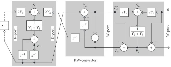
Figure5: FDTD node (left) and a DWG node (right) forming a part of a hybrid waveguide. There is a Kconverter between K- and W-models.Yiare wave admittances of W-lines, K-pipes, and KW-converter between junction nodes.P1andP2are the junction pressures of the K-node and W-node, respectively.

and the recursion in (24) can be expressed inz-domain as

PJ,k+z−2PJ,k=2_Y i

N

i=1

z−1_Y

iPJ,i. (26)

The superposition of the excitation block in (14) and the N-port formulation above completes the formulation of the FDTD model structure. In particular, by settingN = 3 the digital filter structure inFigure 3is obtained.

3.4. Construction of mixed models

An essential difference between DWGs ofFigure 2and FDTD model structures of Figure 3 is that while DWG junctions are connected through two-directional delay lines (W-lines), FDTD nodes have two unit delays of internal memory and delay-free K-pipes connecting ports between nodes. These junction nodes and ports are thus not directly compatible. The next question is the possibility to interface these sub-models. The interconnection of a lossy FDTD model struc-ture and a similar DWG has been tackled in [17]. A proper in-terconnection element (converter) has been proposed for the

resulting hybrid model in this special case. A generalization has been proposed in [18], which allows to make any hybrid model of K-elements (FDTD) and W-elements having arbi-trary wave admittances/impedances at their ports (see also [21]).

Here, we derive how a hybrid model (shown inFigure 5) can be constructed in a 1D waveguide between a K-nodeN1 (left) and a W-nodeN2(right), aligned with the spatial grids k = 1 and 2, respectively. The derivation is based on the fact that the junction pressures are available in both types of nodes, but in the DWG case not at the W-ports.

If N1 andN2 would be both W-nodes (see Figure 8 in the appendix), the traveling wave entering into the nodeN2 could be calculated as

P+

2 =z−1P−1 =z−1

P1−z−1P−2

=z−1_P

1−z−2P−2. (27) Note thatP1is available in the K-nodeN1inFigure 5. Con-versely, if N1 andN2 would be both K-nodes, the junction pressure z−1_P

yt yt yt

w w w

wl wl wl

wl w wl w wl w wl w yt

kw kw wl

kp k kp k kw w wl w yt

kp kp wl

kp k kp k kw w wl w yt

kp kp wl

Figure6: Part of a 2D waveguide mesh composed of (a) K-type FDTD elements (left bottom): K-pipes (kp) and K-nodes (k), (b) W-type DWG elements (top and right): delay-controllable W-lines (wl), W-nodes (w), and terminating admittances (yt), and (c) converter elements (kw) to connect K- and W-type elements into a mixed model.

components within the converter

z−1_P 2=z−1

P+ 2 +P2−

. (28)

Equation (27) may be inserted in (28) to yield the following transfer matrix of the 2-port KW-converter element

P+ 2 z−1_P

2

=

1 −z−2 1 1−z−2 z

−1_P 1 P−

2

. (29)

The KW-converter in Figure 5essentially performs the cal-culations given in (29) and interconnects the K-type port of an FDTD node and the W-type port of a DWG node. The signal behavior in a mixed modeling structure is further in-vestigated in the appendix.

4. IMPLEMENTATION OF MIXED MODELS

The functional equivalence and mixed modeling paradigm of DWGs and FDTDs presented above allows for flexible build-ing of physical models from K- and W-type of substructures. In this way, it is possible to exploit the advantages of each type. In this section, we will explore a simple example of digital waveguide model that shows how the mixed mod-els can be built. Before that, a short discussion on the pros and cons of the different paradigms in practical realizations is presented.

4.1. K-modeling versus W-modeling, pros and cons

An advantage of W-modeling is in its numerical robustness. By proper formulation, the stability is guaranteed also with fixed-point arithmetics [5,19]. Another useful property is the relatively straightforward way of using fractional delays [22] when building digital waveguides, which makes for ex-ample tuning and run time variation of musical instrument models convenient. In general, it seems that W-modeling is the right choice in most 1D cases.

The advantages of K-modeling by FDTD waveguides are found when realizing mesh-like structures, such as 2D and 3D meshes [7,8]. In such cases, the number of unit delays (memory positions) is two for any dimensionality, while for a DWG mesh it is two times the dimensionality of the mesh. A disadvantage of FDTDs is their inherent lack of numeri-cal robustness and tendency of instability for signal frequen-cies near DC and the Nyquist frequency. Furthermore, FDTD junction nodes cannot be made memoryless, which may be a limitation in nonlinear and parametrically varying models.

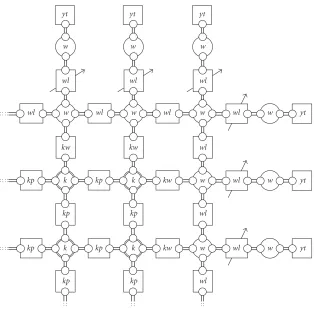
4.2. 2D waveguide mesh case

of a drum or in a 3D case a room enclosed by walls. When there is need to attach W-type termination admittances to the model or to vary the propagation delays within the sys-tem, a change from K-elements to W-elements through con-verters is a useful property. Furthermore, variable-length de-lays can be used, for example, for passive nonlinearities at the terminations to simulate gongs and other instruments where nonlinear mode coupling takes place [23]. The same princi-ple can be used to simulate shock waves in brass instrument bores [24]. In such cases, the delay lengths are made depen-dent on the signal value passing through the delay elements.

InFigure 6, the elements denoted bykpare K-type pipes between K-type nodes. Elementskware K-to-W converters and elementswlare W-lines, where the arrows indicate that they are controllable fractional delays. Elements yt are ter-minating admittances. In a general case, scattering can be controlled by varying the admittances, although the compu-tational efficiency is improved if the admittances are made equal. In a modern PC, a 2D mesh of a few hundred elements can run in real time at full audio rate. By decimated compu-tation, bigger models can be computed if a lower cutoff fre-quency is permitted, allowing large physical dimensions of the mesh.

4.3. Mixed modeling in BlockCompiler

The development of the K- and W-models above has led to a systematic formulation of computational elements for both paradigms and mixed modeling. The W-lines and K-pipes as well as related junction nodes are useful abstractions for a formal specification of model implementation. We have developed a software tool for physical modeling called the BlockCompiler [20] that is designed in particular for flexible modeling and efficient real-time computation of the models. The BlockCompiler contains two levels: (a) model cre-ation and (b) model implementcre-ation. The model crecre-ation level is written in the Common Lisp programming lan-guage for maximal flexibility in symbolic object-based ma-nipulation of model structures. A set of DSP-oriented and physics-oriented computational blocks are available. New block classes can be created either as macro classes composed of predefined elementary blocks or by writing new elemen-tary blocks. The blocks are connected through ports: inputs and outputs for DSP blocks and K- or W-type ports for phys-ical blocks. A full interconnected model is called a patch.

The model implementation level is a code generator that does the scheduling of the blocks, writes C source code into a file, compiles it on the fly, and allows for streaming sound in real time or computation by stepping in a sample-by-sample mode. The C code can also be exported to other platforms, such as the Mustajuuri audio platform [25] and pd [26]. Sound examples of mixed models can be found at http://www.acoustics.hut.fi/demos/waveguide-modeling/.

5. SUMMARY AND CONCLUSIONS

This paper has presented a formulation of a specific FDTD model structure and showed its functional equivalence to the

DWGs. Furthermore, an example of mixed models consist-ing of FDTD and DWG blocks and converter elements is re-ported. The formulation allows for high flexibility in build-ing 1D or higher dimensional physical models from inter-connected blocks.

The DWG method is used as a primary example to the wave-based methods in this paper. Naturally, the KW-converter formulation is applicable to any W-method, such as the wave digital filters (WDFs) [19]. In the future, we plan to extend our examples to include WDF excitation blocks. Other important future directions are the analysis of the dy-namic behavior of parametrically varying hybrid models, as well as benchmark tests for computational costs of the pro-posed structures.

Matlab scripts and demos related to DWGs and FDTDs can be found athttp://www.acoustics.hut.fi/demos/ waveguide-modeling/.

APPENDIX

A. PROOFS OF EQUIVALENCE

The proofs of functional equivalence between the DWG and FDTD formulations used in this article are given below. The approach useful for this can be based on the Thevenin and Norton theorems [27].

A.1. Termination in a DWG network

Passive termination of a DWG junction port by a given ad-mittanceY is equivalent to attaching a delay line of infinite length and wave admittanceY. In the DWG case, this means an infinite long sequence of admittance-matched unit delay lines. Since there is no back-scattering in finite time, we can use the left-side port termination ofFigure 2, with zero vol-ume velocity in input terminal. Thus, admittance filter Y1 is not needed in computation, it has only to be included in making the filter 1/Y_i.

A.2. Termination in an FDTD network

Deriving the passive port termination for an FDTD junc-tion is not as obvious as for a DWG juncjunc-tion. We can ap-ply again an infinitely long sequence of admittance-matched FDTD sections, as depicted inFigure 7on the left-hand side. With the notations given andz-transforms of variables and admittances we can denote

P0=2Y_Y1

iP−1z

−1₊2 Yi

M

i=2

YiPiz−1−P0z−2, (A.1a)

+

P−2

− +

z−1 _z−1

+

P−1

− +

z−1 _z−1

2Y1 + 2Y2

1

Yi

− +

P0

z−1 _z−1

Figure7: FDTD structure terminated by admittance-matched chain of FDTD elements on the left-hand side.

Uext

0 2Y1 + 2Y2

1

Y1+Y2

− +

P1

− +

P−

1 z−1

z−1

P+ 2

2Y2 + 2Y3 ₀

1

Y2+Y3

− +

P2

− +

P−

2

Figure8: Structure for derivation of signal behavior in a DWG network.

k=2,. . .,Nwe get

P−1=P0z−1+P−N−1z−N−P−Nz−N−1. (A.2) WhenN→ ∞, the last two terms cease to have effect onP−1 in any finite time span and they can thus be discarded. When the resultP−1=P0z−1is used in (A.1a), we get

P0=

2Y1

YiP0z −1

z−1₊2 Yi

M

i=2

YiPiz−1−P0z−2, (A.3)

where the first term on the right-hand side can be interpreted as a way to implement the termination as a feedback through a unit delay as illustrated inFigure 3for the left-hand port of the FDTD junction.

A.3. Signal behavior in a DWG network

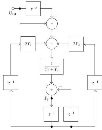
Figure 8illustrates a case where an arbitrarily large intercon-nected DWG network is reduced so that only two scattering junctions, connected through unit delay line of wave admit-tanceY2, are shown explicitly. Norton equivalent sourceUext is feeding junction node 1 and an equivalent termination ad-mittance isY1. Junction node 2 is terminated by a Norton equivalent admittance Y3. Now, we derive the signal prop-agation fromUext to junction pressureP1 and transmission ratio between pressuresP2 andP1. If these “transfer func-tions” are equal for the DWG, the FDTD, and the mixed case with KW-converter, the models are functionally equivalent

Uext

z−2

− +

2_Y1 + 2Y2

1

Y1+Y2 z−1

+ −

z−1

PJ

z−1 _z−1

Figure9: FDTD structure for derivation of volume velocity source (Uext) to junction pressure (PJ) transfer function.

2Y1 + 2Y2

Figure10: FDTD structure for derivation of signal relation between two junction pressures.

0 2Y1 + 2Y2

Figure11: Mixed modeling structure for derivation of DWG to FDTD pressure relation.

FromFigure 8, we can write directly for the propagation of equivalent sourceUextto junction pressureP1as

P1=_YUext 1+Y2.

(A.4)

Signal transmission ratio between P2 and P1 can be de-rived from the following set of equations (A.5a), (A.5b), and (A.5c): equivalence with FDTD and mixed modeling cases.

A.4. Signal behavior in an FDTD network

Using notations inFigure 9, which shows a Norton’s equiva-lent for an FDTD network, we can write

PJ =_YUext

that after simplification yields

PJ =_YUext 1+Y2

, (A.9)

which is equivalent to the DWG form (A.4). Notice that form (1−z−2_{) in feedingU}

extto the node has zeros on the unit cir-cle for anglesnπ(nis integer), compensating poles inherent in the FDTD backbone structure. This degrades numerical robustness of the structure around these frequencies.

which simplifies to

being equivalent to the DWG form (A.7). This completes proving the equivalence of the DWG and FDTD structures.

A.5. Signal behavior in a mixed modeling structure

To prove the equivalence of signal behavior also in the mixed modeling structure ofFigure 5with a KW-adaptor, we have to analyze the junction signal relations in both directions. We first prove the equivalence in the FDTD to DWG direction. According toFigure 5, we can write

P2=

According toFigure 11, we can analyze signal relation-ship in the DWG to FDTD direction by writing

P2= (A.7). This concludes proving the equivalence of the mixed modeling case to corresponding DWG and thus also to FDTD structures.

ACKNOWLEDGMENTS

This work is part of the Algorithms for the Modelling of Acoustic Interactions (ALMA) project (IST-2001-33059) and has been supported by the Academy of Finland as a part of the project “Technology for Audio and Speech Processing” (SA 53537).

REFERENCES

[1] J. L. Kelly and C. C. Lochbaum, “Speech synthesis,” inProc. 4th International Congress on Acoustics, pp. 1–4, Copenhagen, Denmark, September 1962.

[2] N. H. Fletcher and T. D. Rossing, The Physics of Musical In-struments, Springer-Verlag, New York, NY, USA, 2nd edition, 1998.

[3] J. D. Markel and A. H. Gray, Linear Prediction of Speech, Springer-Verlag, New York, NY, USA, 1976.

[4] J. O. Smith, “Physical modeling using digital waveguides,”

Computer Music Journal, vol. 16, no. 4, pp. 74–91, 1992. [5] J. O. Smith, “Principles of digital waveguide models of

musi-cal instruments,” inApplications of Digital Signal Processing to Audio and Acoustics, M. Kahrs and K. Brandenburg, Eds., pp. 417–466, Kluwer Academic Publishers, Boston, Mass, USA, 1998.

[6] M. Karjalainen, V. V¨alim¨aki, and T. Tolonen, “Plucked-string models: From the Karplus-Strong algorithm to digital waveg-uides and beyond,”Computer Music Journal, vol. 22, no. 3, pp. 17–32, 1998.

[7] S. A. Van Duyne and J. O. Smith, “Physical modeling with the 2-D digital waveguide mesh,” inProc. International Computer Music Conference, pp. 40–47, Tokyo, Japan, September 1993. [8] L. Savioja, T. J. Rinne, and T. Takala, “Simulation of room

acoustics with a 3-D finite difference mesh,” inProc. Interna-tional Computer Music Conference, pp. 463–466, Aarhus, Den-mark, September 1994.

[9] L. Savioja,Modeling techniques for virtual acoustics, Ph.D. the-sis, Helsinki University of Technology, Espoo, Finland, 1999. [10] S. D. Bilbao, Wave and scattering methods for the numerical

integration of partial differential equations, Ph.D. thesis, Stan-ford University, StanStan-ford, Calif, USA, May 2001.

[11] J. C. Strikwerda, Finite Difference Schemes and Partial Diff er-ential Equations, Wadsworth and Brooks/Cole, Pacific Grove, Calif, USA, 1989.

[12] L. Hiller and P. Ruiz, “Synthesizing musical sounds by solving the wave equation for vibrating objects: Part 1,”Journal of the Audio Engineering Society, vol. 19, no. 6, pp. 462–470, 1971. [13] L. Hiller and P. Ruiz, “Synthesizing musical sounds by solving

the wave equation for vibrating objects: Part 2,”Journal of the Audio Engineering Society, vol. 19, no. 7, pp. 542–551, 1971. [14] A. Chaigne, “On the use of finite differences for musical

syn-thesis. Application to plucked stringed instruments,” Journal d’Acoustique, vol. 5, no. 2, pp. 181–211, 1992.

[15] M. Karjalainen, “1-D digital waveguide modeling for im-proved sound synthesis,” inProc. IEEE International Con-ference on Acoustics, Speech and Signal Processing, vol. 2, pp. 1869–1872, Orlando, Fla, USA, May 2002.

[16] C. Erkut and M. Karjalainen, “Virtual strings based on a 1-D FDTD waveguide model: Stability, losses, and traveling waves,” inProc. Audio Engineering Society 22nd International Conference on Virtual, Synthetic and Entertainment Audio, pp. 317–323, Espoo, Finland, June 2002.

[17] C. Erkut and M. Karjalainen, “Finite difference method vs. digital waveguide method in string instrument modeling and synthesis,” inProc. International Symposium on Musical Acoustics, Mexico City, Mexico, December 2002.

[18] M. Karjalainen, C. Erkut, and L. Savioja, “Compilation of unified physical models for efficient sound synthesis,” inProc. IEEE International Conference on Acoustics, Speech and Signal Processing, vol. 5, pp. 433–436, Hong Kong, China, April 2003. [19] A. Fettweis, “Wave digital filters: Theory and practice,” Proc.

IEEE, vol. 74, no. 2, pp. 270–327, 1986.

[20] M. Karjalainen, “BlockCompiler: Efficient simulation of acoustic and audio systems,” inProc. 114th Audio Engineering Society Convention, Amsterdam, Netherlands, March 2003, preprint 5756.

[21] M. Karjalainen, “Time-domain physical modeling and real-time synthesis using mixed modeling paradigms,” inProc. Stockholm Music Acoustics Conference, vol. 1, pp. 393–396, Stockholm, Sweden, August 2003.

[22] T. I. Laakso, V. V¨alim¨aki, M. Karjalainen, and U. K. Laine, “Splitting the unit delay-tools for fractional delay filter de-sign,”IEEE Signal Processing Magazine, vol. 13, no. 1, pp. 30– 60, 1996.

[23] J. R. Pierce and S. A. Van Duyne, “A passive nonlinear digital filter design which facilitates physics-based sound synthesis of highly nonlinear musical instruments,”Journal of the Acousti-cal Society of America, vol. 101, no. 2, pp. 1120–1126, 1997. [24] R. Msallam, S. Dequidt, S. Tassart, and R. Causs´e, “Physical

[25] T. Ilmonen, “Mustajuuri—an application and toolkit for in-teractive audio processing,” inProc. International Conference on Auditory Display, pp. 284–285, Espoo, Finland, July 2001. [26] M. Puckette, “Pure data,” inProc. International Computer

Mu-sic Conference, pp. 224–227, Thessaloniki, Greece, September 1997.

[27] J. E. Brittain, “Thevenin’s theorem,” IEEE Spectrum, vol. 27, no. 3, pp. 42, 1990.

Matti Karjalainenwas born in Hankasalmi, Finland, in 1946. He received the M.S. and the Dr.Tech. degrees in electrical engineer-ing from the Tampere University of Tech-nology, in 1970 and 1978, respectively. Since 1980 he has been a professor in acoustics and audio signal processing at the Helsinki University of Technology in the Faculty of Electrical Engineering. In audio technology, his interest is in audio signal processing

such as digital signal processing (DSP) for sound reproduction, perceptually based signal processing, as well as music DSP and sound synthesis. In addition to audio DSP, his research activities cover speech synthesis, analysis, and recognition, perceptual audi-tory modeling and spatial hearing, DSP hardware, software, and programming environments, as well as various branches of acous-tics, including musical acoustics and modeling of musical instru-ments. He has written more than 300 scientific and engineering ar-ticles and contributed to organizing several conferences and work-shops. Professor Karjalainen is Audio Engineering Society (AES) Fellow and Member in Institute of Electrical and Electronics En-gineers (IEEE), Acoustical Society of America (ASA), European Acoustics Association (EAA), International Computer Music As-sociation (ICMA), European Speech Communication AsAs-sociation (ESCA), and several Finnish scientific and engineering societies.

Cumhur Erkut was born in Istanbul, Turkey, in 1969. He received his B.S. and his M.S. degrees in electronics and communi-cation engineering from the Yildiz Techni-cal University, Istanbul, Turkey, in 1994 and 1997, respectively, and the Dr.Tech. degree in electrical engineering from the Helsinki University of Technology (HUT), Espoo, Finland, in 2002. Between 1998 and 2002, he worked as a researcher at the Laboratory