Shift of the mean magnetic field values: Effect of scatter
due to secular variation and errors
Tadahiro Hatakeyama1,2and Masaru Kono2
1Department of Earth and Planetary Science, University of Tokyo, 7-3-1 Hongo, Bunkyo-ku, Tokyo 113-0033, Japan 2Institute for Study of the Earth’s Interior, Okayama University, 827 Yamada, Misasa, Tottori 682-0193, Japan
(Received April 12, 2000; Revised August 4, 2000; Accepted September 25, 2000)
Paleomagnetic data are mostly given in the form of field directions (inclinations and declinations) which depend nonlinearly on the model parameters (Gauss coefficients). Because of this nonlinearity, the means of the data are affected not only by the means of the parameters but also by their fluctuations. Defining the mean directions by the Fisher method decreases this effect but does not completely eliminate it. For various mean fields, we evaluate the effect of secular variation on the means of Fisher-averaged directions by the analytical (Taylor expansion to the second order) as well as by the numerical (Monte Carlo) method. It was shown that a significant amount of offset occurs in the field values because of the fluctuation caused by secular variation. In the case of an inclination anomaly, the effect of secular variation as a function of latitude is antisymmetric about the equator, similar to that of the axial octupole term (g30). We also show that the measurement errors do not induce biases in the mean field data, provided that they are random and isotropic.
1.
Introduction
In the characterization of the global magnetic field, the use of spherical harmonic analysis and description by Gauss coefficients is the standard as this gives a complete and unique representation of the source-free magnetic field (Langel, 1987). In the case of the paleomagnetic field, similar ap-proaches have been sought for a long time (Benkovaet al., 1970; Creeret al., 1973). However, these early efforts were not very satisfactory since they did not take care of the non-uniqueness associated with the inversion of magnetic direc-tion data (Kono, 1976; Proctor and Gubbins, 1990; Hulotet al., 1997).
Modern inversion methods such as stochastic inversion (Jackson, 1979; Gubbins, 1983; Gubbins and Bloxham, 1985) or harmonic splines (Shureet al., 1982) were devel-oped to take care of these problems. These methods apply some physically plausible conditions, so that the solutions are sought within the bounds that such constraints are satisfied. These inversion methods are also powerful in applications where data quality is far from ideal (large errors, poor site distribution, etc.). Gubbins and Kelly (1993), Johnson and Constable (1995, 1997) and Kelly and Gubbins (1997) em-ployed inversion methods adapted to the nonlinear direction data. These authors gave time-averaged magnetic fields for the last 5 million years.
Konoet al.(2000a), however, pointed out that not only the means but also the variances of Gauss coefficients affect the means of nonlinear data, and pointed out that these authors did not properly consider this effect. To avoid the complexity of this problem, Konoet al.(2000a) used only paleointensity
Copy right cThe Society of Geomagnetism and Earth, Planetary and Space Sciences (SGEPSS); The Seismological Society of Japan; The Volcanological Society of Japan; The Geodetic Society of Japan; The Japanese Society for Planetary Sciences.
data in their inversion, which are actually linear data, since information about vector directions is also available for them. This approach is easier but not satisfactory as paleointensity data are much less abundant than paleodirection data.
If we consider the abundance of directional data compared to intensity data, the use of nonlinear data is unavoidable for recovering the paleomagnetic field structure. The sugges-tion by Konoet al.(2000a) is theoretically correct; there are always contributions to the mean of the field values from the fluctuation of the parameters because of the nonlinearity of the data used. However, their discussion and an analyti-cal estimate by Kono (1997a) were based on this effect seen through the simple means of inclinations and declinations. In paleomagnetism, these angles are not usually averaged separately but the mean direction is defined by the method proposed by Fisher (1953), i.e., taking the direction of the sum of the unit vectors representing the direction of individ-ual measurements. This procedure markedly reduces the bias in the mean. So, if the effect of fluctuations is made small enough by taking the Fisher-type means, a reasonable mean field model can still be obtained from the mean direction data assuming one-to-one correspondence between the data and the parameters. To evaluate the relevance of the mean field models thus far proposed, we need a quantitative estimate of the effect of fluctuations on the mean direction in the case of the Fisher averaging procedure.
In this study, we evaluate the effect of scatter on the mean field when calculated by the Fisher method. For this pur-pose, we take a few typical mean field models and assume that the behavior of the parameters (Gauss coefficients) in a long-term secular variation can be modeled by treating them as normal variates having some averages corresponding to the mean field and certain variances. As a theoretical ap-proach, we employ the accurate second-order Taylor
32 T. HATAKEYAMA AND M. KONO: SHIFT OF GEOMAGNETIC FIELD BY PSV
sion. We compare these“analytical”results with the numer-ical ones obtained by generating random models following the assumed distribution of parameters. We also evaluate the effect of errors in measurements of the mean directions and examine whether these effects can be distinguished from the effects of the secular variation.
2.
Taylor Series Expansion of Magnetic Field Data
We can express the three orthogonal components (X,Y
andZ) of the geomagnetic field using a potential obtained by spherical harmonic analysis (see Appendix A.1). These components depend linearly on the parameters of thefield model (Gauss coefficients). Nonlinear quantities, such as direction cosines (x, y, z),field directions (D andI), and virtual geomagnetic pole (VGP), can be described by a com-bination of the linear components (summarized in Appendix A.2 and A.3).
2.1 Expressions for nonlinear data
In general, a nonlinear element of the magneticfield A
(such as inclination or declination) can be expressed by Tay-lor expansion around a reference model m0 (Konoet al.,
2000a)
whereA0is the observation corresponding to the reference
model,
A0=A(m0), (2)
andmis a vector composed of the model parameters (Gauss coefficients), which is a sum of the reference modelm0and
deviation from it
m=m0+m. (3)
The subindices attached to afield value indicate derivatives with respect to the components of modelm; i.e.,Aj,Aj kand
Aj klare, respectively, thefirst, second, and third derivatives of A
is always reserved for representing the value for the reference model. Explicit forms of thefirst and second derivatives of various magneticfield data which are useful in paleomagnetic analyses are given in Appendix A. From (1), the mean and the variance of some component of thefield can be calculated as
Variations in Gauss coefficients in a long-term secular vari-ation can be modeled by assuming that eachmjis an indepen-dent random variable following a normal distribution with the meanμj and the varianceσ2j (Constable and Parker, 1988)
mj ∼N(μj, σ2j). (7)
If the reference model m0 is equated with the mean field
modelμμμμμμμμ= {μj}, eachmj becomes a zero-mean normal variate
mj ∼N(0, σ2j). (8)
Therefore, (5) and (6) are now
E [A]= A0+
As we have assumed normal distribution for each mj, the means and variances of data depend only on even-order derivatives, so that (9) and (10) are valid to the fourth or-der, and the next terms are sixth order inmj. In (9), the first term is due to the mean of the model parameters, while the second and third terms show the effects of the variances of the secular variation model on the meanfield. If we deal only with linear observations (X,Y andZ), these terms do not matter because the second and higher-order derivatives of them are all exactly zero. The above equations indicate that the means of nonlinear data (D,I,. . .) depend not only on the means but are also influenced by the variances of the model parameters (Konoet al., 2000a). This fact complicates the derivation of a time-averagedfield from time-averaged data. It may also affect the stability of the iteration procedures when we solve a nonlinear inverse problem.
In the following analyses, we use the equation of the mean (9) truncated at the second order (i.e., up to the terms withσ2
j) as the“analytical”expression for the nonlinear quantities.
2.2 Expressions for the Fisherian means
The above method can be used to obtain averages of incli-nation and decliincli-nation, separately, but the so-called “mean direction”in paleomagnetism is almost always defined by us-ing the method proposed by Fisher (1953). In this procedure, each directional datum is converted to direction cosines
xn =cosIncosDn, yn =cosInsinDn,
and the best estimate of the mean direction is calculated from theNunit vectors as
¯
whereRis the length of the sum ofNunit vectors,
R=
By dividing both the numerator and denominator of (12) by
N, we see that, for instance, x¯F = Ex/Ef, where Ex = E [x], etc., andEf =
E2
x+E2y+Ez2is the mean displace-ment in anN-step random walk. The mean direction in the sense of Fisher (D¯F andI¯F) is calculated from these as scheme of Taylor expansion applicable to the above form.
In general, a composite function ofm
C(A)=CA(1)(m),A(2)(m),· · ·, (15)
provided that the intermediate functionsA(p)are independent of each other. The expansion (16) is again carried out for the reference model m0, and the value of A(p)(m) is divided
into the part corresponding to the reference model and to the residual
A(p)= A0(p)+A(p). (17) Note that the residual partA(p)not only contains thefirst order but also all the higher-order terms inmjas shown in (1). Equation (16) may be further reduced by Eq. (1). Here, we consider the case where the intermediate functions are the means of the direction cosines
A=Ex,Ey,Ez
. (18)
The expansions for these intermediate functions were ob-tained from Eq. (9). Because the lowest-order term inA(p) is proportional toσ2
j (i.e., nofirst-order term), the expansion form, accurate up to the second order, is simply
¯
With this form, we calculate the effect of the geomagnetic secular variation (in Section 3) and the measurement errors (in Section 4) in the Fisher-mean directions. The explicit forms are listed in Appendix A.4.
3.
Effect of Secular Variation on the Mean Field
Values
With the appropriate Taylor expansion forms, we can ana-lytically evaluate the effect of scatter in the data on the mean values offield directions and direction cosines. The scatter in the data are caused either by secular variation of the magnetic
field or by errors in various phases of the treatments used to recover thefield directions. We will consider only the effect of secular variation in this section and treat the errors in the next section.
Analytical estimation is based on the Taylor series ex-pansion up to second order, using the Fisher-averaging pro-cedure. To supplement the analytical estimates, numerical calculations were done with a 105set of randomly generated Gauss coefficients. This number seems to be enough to sat-isfactorily represent the distribution of the assumed secular variation. Comparison between these two calculations gives estimates of the effects due to the fourth and higher-order terms.
We consider two types of mean field models; the geo-centric axial dipole (GAD, in Subsection 3.2)field, and two nonaxisymmetricfield models (in Subsection 3.3). In each case, the variances of Gauss coefficients are assumed to de-pend only on the degree of the spherical harmonic and not on the order. In a few cases, some of the non-dipole terms were allowed to deviate from the general trend (in Subsec-tion 3.4). Because the IGRF 1995 (Barton, 1997) was used as one of the non-axisymmetric meanfields, all the models were calculated up to the maximum degree of 10 (max=10). 3.1 Model for secular variation
Paleomagnetic secular variation (PSV) models have been proposed by various authors (e.g. Cox, 1970; McFaddenet al., 1988). In this paper, we adopt a model similar to those proposed by Constable and Parker (1988) and by Kono and Tanaka (1995). These models are based on the observed exponential decay of the power of the geomagneticfield with a spherical harmonic degree. For the presentfield, an almost
flat spectrum is observed at the core-mantle boundary (CMB) (Langel and Estes, 1982). This feature is also seen in the self-consistent three-dimensional geodynamo simulation models (e.g. Glatzmaier and Roberts, 1995; Konoet al., 2000b).
In the model of Constable and Parker (1988), the power in a degree is divided equally into harmonics of different orders, so that the variances of a degreeGauss coefficient are given as
where a andc are the radii of the Earth and its core, re-spectively. Constable and Parker (1988) estimated the value of αfor the presentfield as 27.7μT, excluding the dipole (=1) terms. A few other terms were permitted to behave differently in the model of Constable and Johnson (1999).
In this paper, we use Eq. (20) with various values ofα to define the variances of Gauss coefficients, including the dipole terms. In paleosecular PSV models, we implicitly assume that the statistical properties of thefield models are well sampled by observations for a long period of time. In the numerical calculations, we use 105 random models to
34 T. HATAKEYAMA AND M. KONO: SHIFT OF GEOMAGNETIC FIELD BY PSV
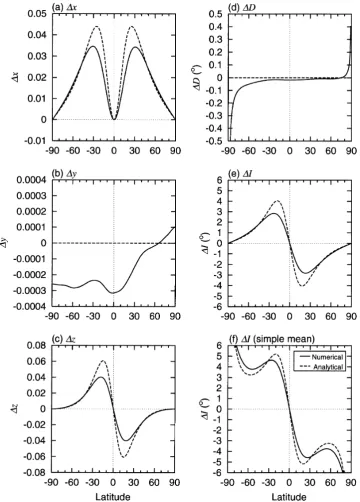
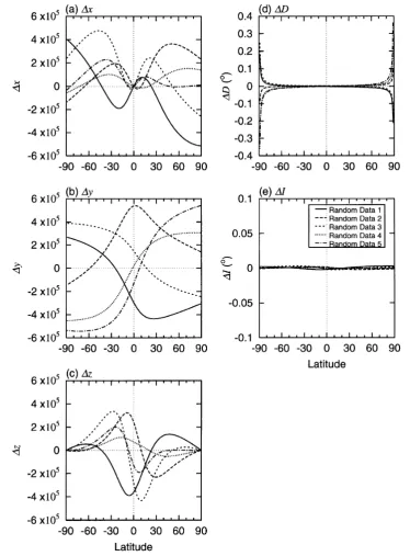
Fig. 1. Latitude dependency of the biases; (a)x, (b)y, (c)z, (d)Dand (e)I; by numerical (solid lines) and second-order analytical (dashed) calculation and (f)Icalculated by a simple averaging method (like in Kono, 1997a). The meanfield is due to GAD (g0
1 = −30.0μT) and a PSV model (α=30.0μT in Eq. (20)). Note that the values ofyandDdue to the random data set (N=105) are very small and their analytical value is exactly zero.
possible ranges offluctuation.
3.2 Fluctuations about the geocentric axial dipolefield
As an example of the simplest model, the GAD field (g0
1 = −30μT) was taken as the meanfield. In this case,
thefluctuations around the mean with the form (20) produce only an axisymmetric effect. Figure 1 shows the deviations of the means of direction cosinesx,y,zand anglesDandI
from the axial dipolefield values. Biases estimated analyti-cally (by Taylor expansion) and numerianalyti-cally (by 105random
models) are shown. For Figs. 1(a)–(e), the mean values were
determined by the Fisher (1953) method, i.e., the direction of the sum of unit vectors. Figure 1(f), on the other hand, gives the deviation of the simple mean of the inclination from the axial dipole value.
It can be seen that there are indeed biases due to the pres-ence offluctuations (such as secular variation), except forD
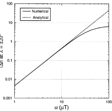
Fig. 2. αdependency of|I|at the latitude of 20◦N and S with the same parameters in Fig. 1, suggesting that the second-order accurate expression (A.24, dashed line) of|I|always overestimates the numerical value (solid).
on the equator. By simple averaging (Fig. 1(f)) the values of Iare significantly higher than those of the Fisherian mean (Fig. 1(e)). Figure 1(f) also shows that a simple mean makes I much larger near the poles because of the singularity in its definition (Kono, 1997a).
The inclination differences in the case of the GAD mean
field have a trend that the absolute value of inclination be-comes smaller everywhere on the Earth’s surface. The dif-ference becomes larger with an increase in amplitude (α) of the secular variation. It is only about 0.5◦whenα=10μT (Fig. 2), which can easily be buried by the usual errors in pa-leomagnetic data. The bias becomes significant for largerα (1.5◦for 20μT and 4◦for 40μT). We can conclude that the scatter of data due to secular variation will affect the mean values of observed inclinations at these latitudes ifαis 20μT or larger.
The Taylor expansion to the second order (A.24) gives the correct magnitude of inclination bias up to aboutα=20 μT. For larger values ofα, the analytical method gives larger estimates than those obtained by random numerical models. In x, z, I (Fisher means), analytical values always produce overestimates, whileI, based on a simple average, is larger or smaller than the numerical estimate depending on the latitude. The difference between the two estimates are about 40% or less whenα=30μT (Fig. 2).
3.3 Fluctuation about non-axisymmetric meanfields
Effects of the secular variation are also examined for two non-axisymmetric meanfields; IGRF 1995 (Barton, 1997) and the time-averaged normal-polarity field model for the last 5 million years (JC97N) given by Johnson and Constable (1997). The IGRF 1995 model actually shows an instanta-neousfield containing both the mean and thefluctuation parts, but we use it as an example of afield with large non-dipole components compared to JC97N in which the axial dipole component is much more dominant.
Declination is not a well-defined quantity at very high latitudes (|I| ∼90◦), because the expression forDbecomes singular at the poles (see Kono, 1997a, b). In reality,|D|is
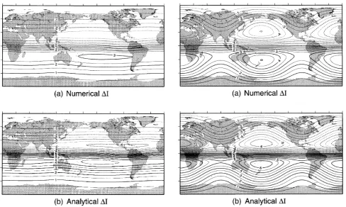
Fig. 3. Mapping of numerical (a) and second-order analytical (b)Iwith the IGRF 1995 meanfield and a PSV model of (20) withα=30.0μT.
less than 0.5◦almost everywhere except in the close vicinity of the poles (cf. Fig. 1(d)). Here we only show the maps of inclination offsetI for the meanfields of IGRF 1995 (Fig. 3) and JC97N (Fig. 4) with a variation ofα=30.0μT. In both cases, the contour on which inclination offset van-ishes (I = 0◦) almost coincides with the geomagnetic equator andI is negative (positive) when the value of I
is positive (negative). Therefore, it can be concluded that the geomagnetic secular variation makes the absolute value of inclination smaller almost everywhere on the Earth’s surface (see also Fig. 1(e)). Furthermore, the features of the mag-neticfield derived from second-order analytic results is very similar to those obtained by numerical calculations. The an-alytical expression overestimates the bias in a similar way to the case of the GAD meanfield. The difference between analytical and numerical estimates becomes conspicuous at sites where the absolute value of inclination is more than 40◦ (|I| 2◦).
36 T. HATAKEYAMA AND M. KONO: SHIFT OF GEOMAGNETIC FIELD BY PSV
Fig. 4. Mapping of numerical (a) and second-order analytical (b)I. The meanfield is the result of Johnson and Constable (1997) from paleomag-netic data in the normal periods for the last 5 Ma as the meanfield, and the PSV model is the same as in Fig. 3.
3.4 Effect of (2,1) harmonics
From the latitude dependence of scatter of the field or the VGP components, Kono and Tanaka (1995) and Kono (1997a, b) concluded that the variation of the quadrupolar terms g1
2 andh 1
2 should be a few sizes larger in amplitude
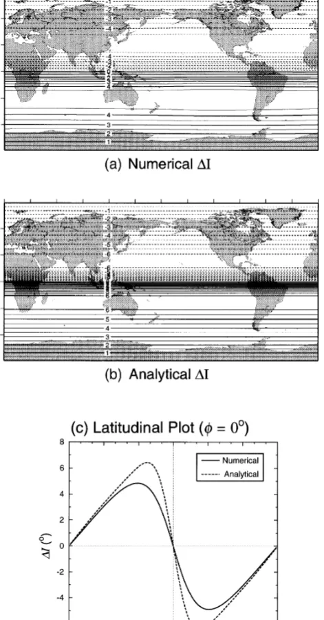
than the general trend given by (20). We evaluate the effect of large (2,1) terms on the mean inclinations. Figure 5 shows the contour map ofIcorresponding to a model which is the same as the axially symmetric model shown in Fig. 1, except that the standard deviation ofg1
2 is made three times larger,
as is given by (20). Four (positive and negative) extrema are shown in theI map, which correspond to theflux patches of theZ field due tog12.
Figure 6 shows the map ofI with a secular variation model in which both of the (2,1) harmonics have larger am-plitudes offluctuation; i.e.,σg1
2 =σh 1
2 =3σ2. In this case,
the effect becomes axisymmetric because the sum ofg1 2 and
h1
2 contributions is a constant of longitude (Kono, 1997b).
The total amount of secular variation is larger in this model compared to 3.2, so that theI is much larger. The latitudi-nal plot (Fig. 6(c)) indicates that the maximum of inclination bias appears at a latitude (about 30◦) which is higher than in the original PSV model (about 20◦, Fig. 1(e)). The reason for this shift seems to be because thefield due to a combina-tion ofg1
2andh 1
2has nodes at the north and south poles and
at the equator. Therefore, the effect of the secular variation by enhancedg1
2 andh 1
2is large at middle latitude which is
higher than the peak by a PSV model following Eq. (20).
Fig. 5. Mapping of numerical (a) and second-order analytical (b)Iwith the meanfield of GAD (g0
1 =30.0μT) and variances from a secular variation model following (20) withα=30μT excludingσg1
2=3σ2.
4.
Effects of Measurement Errors on the Mean
Di-rection
In paleomagnetic studies, the data are inevitably contam-inated by some amount of experimental errors, even if we collect and measure the samples very carefully. These errors are due to many causes; orientation errors during sampling and cutting, shape anisotropy of samples, heterogeneity of magnetization in a specimen, errors of setting in the mag-netometer, errors in the measurements, and so on. Here we omit systematic errors (such as is caused by a strong local magnetic anomaly at sampling sites, or the inability to re-store the original bedding plane), and only consider random errors in each measurement.
By excluding the possibility of systematic errors, we can assume that the errors of the measured componentsX,Yand
Z are mutually independent and zero-mean normal variates. It seems reasonable to assume that the standard deviations in individual components are proportional to its intensity
σX =σY =σZ =s F, (21)
wheresis a constant. (This assumption, in effect, is based on the experience that the source of the largest errors in pa-leomagnetism of volcanic rocks is the orientation errors.)
In the expansion of the means defined by the Fisher proce-dure (A.24), all the second-order terms (A.26) vanish. Thus, the relevant forms of expansion are
¯
xF =
X F +O(s
4), y¯
F =
Y F +O(s
Fig. 6. Mapping of numerical (a) and second-order analytical (b)I, and their sectoral section atφ = 0◦ (c). The mean and variances of Gauss coefficients are the same as in Fig. 5 excludingh1
2as well asg 1 2 (σg1
2=σh 1 2=
3σ2).
¯
zF =
Z F +O(s
4), D¯
F =tan−1
Y X +O(s
4),
¯
IF =tan−1
Z
√
X2+Y2 +O(s
4). (22)
These indicate that the means of the data are not affected by the presence of scatter due to experimental errors, at least to this order.
To show that these analytical conclusions are correct, de-viations from the meanfield values (D,I,x,yand z) were obtained by the random data set (N =105), and
the results are shown in Fig. 7 in which the mean field is GAD ands=0.1 (10% of the total intensity, which is large for usual experimental situations). As can be seen from this
figure, the difference in the means is negligibly small which is in agreement with the above analysis. The small differ-ences shown in this figure are likely to be caused by the incompleteness of the random models, becausefive different random data sets gave quite different results. From these, we can conclude that if we make adequate observations at each site, there will be no bias to the mean direction due to the experimental errors, provided that the errors are not system-atic. Note that this conclusion applies only to the Fisherian means; a significant amount of shallowing results from the scatter due to errors if a simple mean of inclination is taken (e.g., Kono, 1997a). Observational errors also increase the scatter in the data compared to the case with only secular variation.
It is remarkable that the (non-systematic) measurement errors do not cause biases in the means of thefield directions. This is quite different from the behavior of the scatter caused by secular variation. In retrospect, it is quite reasonable that the experimental errors do not induce bias in the meanfield direction, since the Fisher method was created to obtain the most likely estimate of the magnetization direction when data contain random errors (Fisher, 1953). This feature, however, does not apply to secular variation because it generates non-random scatter.
5.
Discussion
5.1 Far side effectPrevious paleomagnetic studies (Wilson, 1970, 1971) sug-gested that observed inclination is shallower than that pro-duced by the GADfield everywhere in the world. This effect is most prominently seen in the Northern Hemisphere. The VGPs for these data are located on the far side of the ge-ographic North Pole. For example, the lava data set from Hawaii indicates that the inclination is 9◦shallower than the GAD, resulting in an offset of 5◦ of the mean VGP from the North Pole (Tanaka, 1999). Combining a small amount of Southern Hemisphere data, Wilson (1970) concluded that this effect can be attributed to the offset of the axial dipole from the geocenter. Equivalently, the“shallow inclination”
or“far side effect”can also be explained by the existence of a non-zero axial quadrupolefield (g0
2) which has the same
sign as that ofg0 1.
With the addition of more data from the Southern Hemi-sphere, however, it became apparent that the addition of the quadrupole term cannot completely explain the inclination anomalies. Indeed, McElhinnyet al.(1996) showed that the inclination anomaly with respect to the GAD value has an asymmetric component. They explained this by introducing the non-zero octupole term (g03), in addition to the dipole and quadrupole in the time-averagedfield, as the inclination anomaly caused byg20is symmetric, while that caused byg30
is antisymmetric about the Equator. We have shown, how-ever, that the effect of random secular variation is similar to that of persistent g0
3 in creating an inclination anomaly
antisymmetric about the Equator (Fig. 1(e)). Thus, the in-clination anomaly observed for the last 5 Ma (McElhinny
38 T. HATAKEYAMA AND M. KONO: SHIFT OF GEOMAGNETIC FIELD BY PSV
Fig. 7. (a)x, (b)y, (c)z, (d)Dand (e)Iby measurement error withs=0.1. There are 5 curves by 105random normal distribution data sets generated by different seeds. They indicate that the amount of random data (N=105) is not enough to see the effect of the measurement errors and, even if it exists, it is much smaller than these shown values.
g0
1+g02+g30(McElhinnyet al., 1996) or byg01+g20combined
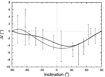
with the effect of secular variation (Fig. 8). In the present case, it is not possible to choose the most probable model from thefit shown in Fig. 8 alone. But it may be important that the observed asymmetry does not necessarily mean the existence of the octupole term.
5.2 Effects of the secular variation and measurement errors on nonlinear inversion
In this study, we considered the effects of variances due to two sources; geomagnetic secular variation and measure-ment error. From the foregoing analyses, it can be concluded
that secular variation really influences the mean directions, but the errors do not change the means. The effect of the geomagnetic secular variation is to make the absolute value of observed inclination smaller everywhere.
direc-Fig. 8. Inclination anomalyI for the normal polarity data (the mean and the 95% confidence interval) of the last 5 Ma (McElhinnyet al., 1996). Dashed curve shows their best estimate withg0
2/g 0
1 = 0.043,
g03/g10 =0.017,g40/g01 = −0.008. Solid curve indicates an example of thefit withg0
2/g01 plus the effect of secular variation expressed by α=0.6|g0
1|.
tions significantly, even when the mean directions are defined as the best estimate of Fisher (1953). The neglect of this ef-fect will result in the estimates of nondipole components with larger errors. Therefore, it is possible that the time-averaged
field may be characterized by parameters somewhat different from those given by their results.
Considering these effects, we can define a new inversion method to seek the time-averaged geomagneticfield and its variances (i.e. PSV) from paleomagnetic data. The mean directions of the observed paleomagnetic data depend on the mean Gauss coefficients as well as on their change due to PSV. The observation equation for the mean direction (or the direction cosines) at a sitei can be obtained from Eq. (A.24) as
Ai = fi(μμμ, σσσσσσσσ),μμμμμ (23) where we take the means{μj}and the variances{σj}of Gauss coefficients as the model parameters to be determined.
In addition, we can define another equation to show the relation between the variances of the parameters and the vari-ances of the observations. The equation for varivari-ances (or standard deviations) depends on the means as well as the variances of Gauss coefficients and the measurement errors
Vi =gi(μμμμμμμμ, σσσσσσσσ,e). (24)
It is necessary to solve (23) and (24) simultaneously in order to properly account for the means and variances of the data. Up to now, such inversion was done only for the linear case (Konoet al., 2000a), but a solution for the nonlinear data set is also required.
5.3 Robustness of the present results
We have obtained the expressions which indicate the effect of scatter caused by secular variation of the magneticfield on the mean values offield data. It was shown that the effect was not negligible; indeed a considerable amount of offset was observed in the mean values of inclination and other field elements. However, in order to derive workable formulas, it was necessary to make a few assumptions about thefield behavior. Thus, the relevance of the present results in secular
variation analysis depends on the validity of the assumptions we employed in deriving the expressions.
We would argue that the assumptions employed are quite reasonable and, moreover, the results do not critically depend on the details of the assumptions. First of all, it is quite certain that there werefluctuations in thefield elements with time; there is no doubt that the secular variation of the magnetic
field occurred with considerable amplitudes. Secondly, the assumption of normal distribution of Gauss coefficients was used more for the convenience of calculation. The Taylor ex-pansion method developed by Kono and Tanaka (1995) and following papers is quite general and applies to any distribu-tions if the existence of low-degree moments (e.g. the mean and variance) can be assumed. Thirdly, using essentially the same assumptions, Constable and Parker (1988) and others (Kono and Tanaka, 1995; Kono, 1997a, b; Constable and Johnson, 1999) obtained reasonable results in the analysis of paleosecular variation in the last 5 Ma, which indicates that it is at least permissible. Lastly, Konoet al.(2000b) showed that numerical dynamo simulation results suggests that the distribution of Gauss coefficients of low degrees are indeed quite similar to normal distribution.
It is impossible at the present stage to convincingly show which distribution is more appropriate to describe thefl uc-tuating Gauss coefficients because of the secular variation. However, it may be reasonable to consider that the distri-bution ofgm orhm is effectively bounded in some interval and that it is not skewed. This makes modeling by normal distribution quite appropriate. Moreover, if the distribution of Gauss coefficients deviates from the normal distribution, the nonlinear effects will be larger than those we derived be-cause the effect of the third (skewness) and fourth moment may not be neglected.
6.
Conclusions
We have quantitatively evaluated the effect of geomag-netic secular variation and measurement errors on the mean directions. If the measurement errors are not systematic, i.e., truly random and isotopic, they do not affect the mean direc-tions but make the variances larger. Thefluctuations in the model due to PSV change the mean directions in which the absolute inclination becomes smaller than that for the mean
field. For example, in a PSV model withα=30.0μT,I
is a few degrees at low to middle latitude sites. In the case where the mean field is the GAD, this inclination anomaly is antisymmetric about the Equator, which is similar to that caused by the non-zero mean value of the axial octupole (g0
3).
It is possible that theg0
3 term reported from the analysis of
secular variation data (e.g., McElhinnyet al., 1996) is partly attributable to this effect. We cannot ignore this effect when we seek the time-averagedfield by nonlinear inversion from paleomagnetic data.
40 T. HATAKEYAMA AND M. KONO: SHIFT OF GEOMAGNETIC FIELD BY PSV
of the biases due to the PSV are very well reproduced by the analytical method in the distribution over the globe, in-dicating the usability of the second-order Taylor expansion approximation.
Acknowledgments. We thank Yozo Hamano and Hidefumi Tanaka for useful discussions. We also thank Michael McElhinny and Hideo Tsunakawa for constructive criticism. T. Hatakeyama was supported by a Japan Society for Promotion of Science Research Fellowship for Young Scientists. Part of this study was supported by a Grant-in-Aid for Scientific Researches (No. 10440124).
References
Barton, C. E., International Geomagnetic Reference Field: The seventh generation,J. Geomag. Geoelectr.,49, 123–148, 1997.
Benkova, N. P., N. V. Adam, and T. N. Cherevko, Application of spherical harmonic analysis to magnetic declination data,Geomagn. Aeron.,10, 673 (Engl. Trans. 527–532), 1970 (in Russian).
Constable, C. G. and C. L. Johnson, Anisotropic paleosecular variation models: implications for geomagneticfield observables,Phys. Earth Planet. Inter.,115, 35–51, 1999.
Constable, C. G. and R. L. Parker, Statistics of the geomagnetic secular variation for the past 5 m.y.,J. Geophys. Res.,93, 11569–11581, 1988. Cox, A. V., Latitude dependence of the angular dispersion of the
geomag-neticfield,Geophys. J. R. astr. Soc.,20, 253–269, 1970.
Creer, K. M., D. T. Georgi, and W. Lowrie, On the representation of the Quaternary and late tertiary geomagneticfields in terms of dipoles and quadrupoles,Geophys. J. R. astr. Soc.,33, 323–345, 1973.
Fisher, R. A., Dispersion on a sphere,Proc. R. Soc. Lond.,A217, 295–305, 1953.
Glatzmaier, G. A. and P. H. Roberts, A three-dimensional self-consistent computer simulation of a geomagneticfield reversal,Nature,377, 203–
209, 1995.
Gubbins, D., Geomagneticfield analysis—I. stochastic inversion,Geophys. J. R. astr. Soc.,73, 641–652, 1983.
Gubbins, D. and J. Bloxham, Geomagneticfield analysis—III. Magnetic
fields on the core-mantle boundary,Geophys. J. R. astr. Soc.,80, 695–713, 1985.
Gubbins, D. and P. Kelly, Persistent patterns in the geomagneticfield over the past 2.5 Myr,Nature,365, 829–832, 1993.
Hoffman, K. A., Dipolar reversal states of the geomagneticfield and core-mantle dynamics,Nature,359, 789–794, 1992.
Hulot, G., A. Khokholov, and J.-L. Le Mouel, Uniqueness of mainly dipolar¨
magneticfields recovered from directional data,Geophys. J. Int.,129, 347–354, 1997.
Jackson, D. D., The use ofa prioridata to resolve non-uniqueness in linear
inversion,Geophys. J. R. astr. Soc.,57, 137–157, 1979.
Johnson, C. L. and C. G. Constable, The time-averaged geomagneticfield as recorded by lavaflows over the past 5 Myr,Geophys. J. Int.,122, 488–519, 1995.
Johnson, C. L. and C. G. Constable, The time-averaged geomagneticfield: global and regional biases for 0–5 Ma,Geophys. J. Int.,131, 643–666, 1997.
Kelly, P. and D. Gubbins, The geomagneticfield over the past 5 Myr, Geo-phys. J. Int.,128, 315–330, 1997.
Kono, M., Uniqueness problems in their spherical harmonic analysis of the geomagneticfield direction data,J. Geomag. Geoelectr.,28, 11–29, 1976. Kono, M. Paleosecular variation infield directions due to randomly varying
Gauss coefficients,J. Geomag. Geoelectr.,49, 615–631, 1997a. Kono, M. Distributions of paleomagnetic directions and poles,Phys. Earth
Planet. Inter.,103, 313–327, 1997b.
Kono, M. and O. Hiroi, Paleosecular variation offield intensities and dipole moments,Earth Planet. Sci. Lett.,139, 251–262, 1996.
Kono, M. and H. Tanaka, Mapping the Gauss coefficients to the pole and the models of paleosecular variation,J. Geomag. Geoelectr.,47, 115–130, 1995.
Kono, M., H. Tanaka, and H. Tsunakawa, Spherical harmonic analysis of paleomagnetic data: the case of linear mapping,J. Geophys. Res.,105, 5817–5833, 2000a.
Kono, M., A. Sakuraba, and M. Ishida, Dynamo simulation and paleosecular variation models,Phil. Trans. R. Soc. Lond.,A358, 1123–1139, 2000b. Langel, R. A., The mainfield, inGeomagnetism, vol. 1, edited by J. A.
Jacobs, pp. 249–512, Academic Press, London, 1987.
Langel, R. A. and R. H. Estes, A geomagneticfield spectrum,Geophys. Res. Lett.,9, 250–253, 1982.
McElhinny, M. W., P. L. McFadden, and R. T. Merrill, The time-averaged paleomagneticfield 0–5 Ma,J. Geophys. Res.,101, 25007–25027, 1996. McFadden, P. L., R. T. Merrill, and M. W. McElhinny, Dipole/quadrupole family modeling of paleosecular variation,J. Geophys. Res.,93, 11583–
11588, 1988.
Proctor, M. R. E. and D. Gubbins, Analysis of geomagnetic directional data,
Geophys. J. Int.,100, 69–77, 1990.
Shure, L., R. L. Parker, and G. E. Backus, Harmonic splines for geomagnetic modelling,Phys. Earth Planet. Inter.,28, 215–229, 1982.
Tanaka, H., Circular asymmetry of the paleomagnetic directions observed at low latitude volcanic sites,Earth Planets Space,51, 1279–1286, 1999. Wilson, R. L., Permanent aspects of the Earth’s non-dipole magneticfield over upper tertiary times,Geophys. J. R. astr. Soc.,19, 417–437, 1970. Wilson, R. L., Dipole offset—The time average palaeomagneticfield over
the past 25 million years,Geophys. J. R. astr. Soc.,22, 491–504, 1971.
Appendix A. Derivatives of Various Field Components
The derivatives of paleomagnetic data with respect to Gauss coefficients have been described by various authors (e.g., Constable and Parker, 1988; Kono and Tanaka, 1995; Kono and Hiroi, 1996; Kono, 1997a, b). However, in many cases, these expressions were given in a form applicable to some specific model (e.g., near GAD), and the notations also vary greatly in each case. For the sake of convenience, we give here the complete form of derivatives of the first and second order. A.1 The linear components of the geomagnetic field
The magnetic field outside the Earth’s core can be described by a scalar potential. The potentialW at a point (r, θ, φ), whereris the radius,θis the colatitude, andφis the longitude, is given by
W =a
max
=1
m=0 a
r
+1
(gmcosmφ+hmsinmφ)Pm(cosθ), (A.1)
wherePmis the Schmidt-normalized Legendre function,gmandhm are Gauss coefficients, andmaxis the maximum degree at which spherical harmonics are truncated. The modelmis a vector formed by arranging the Gauss coefficients by degree and order
m=g01,g11,h11,g20,g21,h12, . . .T. (A.2) Its components will be designated by a single suffix j (j =1, . . . , max(max+2)), such asmj, rather than byandm.
The three components of the magnetic field at some point over the surface of the Earth can be derived from the potential as
X =
j
Xjmj, Y =
j
Yjmj, Z =
j
Zjmj, (A.3)
whereXj,Yj,Zjare functions of position (θ,φ)
Xj =
d Pm dθ
cosmφ
sinmφ
, Yj =
m Pm
sinθ
sinmφ
−cosmφ
, Zj = −(+1)Pm
cosmφ
sinmφ
. (A.4)
The choice ofφdependence is determined by whethermjisgmorhm. Obviously, the three components (X,Y,Z) are linear in Gauss coefficients, andXj,Yj,Zj are their derivatives with respect to a Gauss coefficientmj.
Any other field component, either linear or nonlinear, can be written by a combination of these three components (in some cases, the coordinates of the positionr, θ, φare also needed).
A.2 Nonlinear field elements
In paleomagnetism, data are mostly given by two angles, inclinationIand declinationD. In paleointensity experiments, the total intensityFis determined. These quantities are related to the three components as
I =tan−1
Z H
, D=tan−1
Y X
, F= X2+Y2+Z2, (A.5)
whereH =√X2+Y2. The first and second derivatives of these quantities are
∂I
∂mj =
H2Zj−Z(X Xj+Y Yj)
F2H ,
∂2I
∂mj∂mk
= 1
F4H3
(F2+2H2)Z(X Xj+Y Yj)(X Xk+Y Yk)−F2H2Z(XjXk+YjYk)
+H2(Z2−H2)!(X Xj+Y Yj)Zk +(X Xk+Y Yk)Zj "
−2H4Z ZjZk
, ∂D
∂mj
= X Yj−Y Xj
X2+Y2 ,
∂2D
∂mj∂mk
= −(X Xk+Y Yk)(X Yj−Y Xj)+(X Xj+Y Yj)(X Yk−Y Xk)
H4 ,
∂F
∂mj =
Gj
F ,
∂2F
∂mj∂mk
= Gj k
F − GjGk
F3 , (A.6)
whereH =√X2+Y2is the horizontal component andG=F2/2,G
j =X Xj+Y Yj+Z Zj, etc. For direction cosines,
x=cosIcosD= X
F, y=cosIsinD= Y
F, z=sinI = Z
42 T. HATAKEYAMA AND M. KONO: SHIFT OF GEOMAGNETIC FIELD BY PSV
thefirst and second derivatives ofxare ∂x
∂mj =
Xj
F − X Gj
F3 ,
∂2x
∂mj∂mk
= − 1
F3(XjGk+XkGj+X Gj k)+
3X GjGk
F5 ,
∂3x
∂mj∂mk∂ml
= − 1
F3(XjGkl+XkGjl+XlGj k)
+ 3
F5
XjGkGl+XkGjGl+XlGjGk+X(Gj kGl+GjlGk+GjGkl)
− 15
F7X GjGkGl. (A.8)
Derivatives ofyandzcan be obtained by replacingXbyY or Z.
A.3 Virtual geomagnetic pole (VGP) and its moment
In many cases, VGPs or virtual dipole moments (VDMs) are used in place offield elements because the concept of the dipole is global and suitable for worldwide comparison. The expressions for VGP and VDM have been already reported (Kono and Tanaka, 1995; Kono and Hiroi, 1996; Kono, 1997a). The colatitude (θp) and longitude (φp) of VGP are given by
θp=cos−1
U
, φp=tan−1
, (A.9)
where
U = X2+Y2+(Z/2)2,
= −Xcosθcosφ−Ysinφ+1
2Zsinθcosφ, = −Xcosθsinφ+Ycosφ+1
2Zsinθsinφ, =Xsinθ+ Z
2 cosθ. (A.10)
Thefirst and second derivatives ofθpandφpare
∂θp
∂mj
= 1
T2+2T
Tj−T2j
,
∂2θ
p
∂mj∂mk =
1
T2+22T3
T2T2+2Tj k −3T2+2TjTk
+2T4jk+T2
T2−2 Tjk+Tkj
, ∂φp
∂mj
= 1
2+2
j−j
,
∂2φ
p
∂mj∂mk
= 1
2+22
(jk−jk)−(2−2)(jk+kj)
, (A.11)
where
T = U2−2= #
X2cos2θ+Y2+ Z 2
4 sin
2θ−X Zcosθsinθ (A.12)
andj,k,j,k,jandkare their derivatives, as
j= −Xjcosθcosφ−Yjsinφ+ 1
2Zjsinθcosφ. (A.13)
TjandTj k are defined as
Tj=T ∂T
∂mj
=X Xjcos2θ+Y Yj+ 1 4Z Zjsin
2θ−1
2
XjZ+X Zj
cosθsinθ,
Tj k = ∂T
j
∂mk
=XjXkcos2θ+YjYk+ 1
4ZjZksin
2θ−1
2
XjZk+XkZj
andTkis similar toTj.
The VDM can be calculated as
M =a3U =a3 X2+Y2+(Z/2)2, (A.15)
To express the VDM in the usual unit of Am2, it is necessary to multiply the right-hand side by a factor of 4π/μ
0 =107.
Thefirst and second derivatives of the elements of VGP are
∂M
As was the case in paleomagnetic directions, the mean of the VGPs is defined by summing the unit vector in the direction of the individual VGP. Thus, we need the expressions for the direction cosines (ξp,ηp,ζp) of the pole:
whereandare defined in (A.10). Thefirst and second derivatives ofξpcan be obtained as
∂ξp
The derivatives ofηpandζpcan be obtained by changing the terms concerned with the numerators of Eq. (A.17). A.4 Mean directions defined by Fisher’s method
The Fisherian means of nonlinear data can be expanded following the general method given by Eq. (19). Specifically, we treat the nonlinear quantitiesx¯F,y¯F,z¯F,D¯F, andI¯Fas functions ofEx,Ey, andEz. For instance, for the Fisherian mean
As usual, the suffix 0 indicates that the values are to be evaluated for the reference modelm0. The partial derivatives can be
calculated from (12),
On the other hand, the deviations of the means direction cosines are given by (9)
Ex=
It can be shown from (A.8) that
X∂
Thefinal forms of the Fisher-mean direction cosines and directions, accurate to second order, are
44 T. HATAKEYAMA AND M. KONO: SHIFT OF GEOMAGNETIC FIELD BY PSV
¯
yF =y0+
j
Y G2j F5 −
YjGj
F3
0
σ2
j +O(σ
4
j),
¯
zF =z0+
j
Z G2j F5 −
ZjGj
F3
0
σ2
j +O(σ
4
j),
¯
DF =D0+
j
(XjY −X Yj)Gj
F2H2
0
σ2
j +O(σ
4
j),
¯
IF =I0+
j
Gj(Z(X Xj+Y Yj)−H2Zj)
F4H
0
σ2
j +O(σ
4
j). (A.24)
A.5 Derivatives with respect to the linear componentsX,YandZ
In order to consider only the effect of experimental errors, we canfix thefield model to the reference modelm0, which
means that there is no contribution from thefluctuation of thefield model itself. In this case, the observed linear elements can be expressed as X = X0+X, etc., where X0is the value corresponding to thefield model andX is the error in
measurement. Thus, we can treat the three orthogonal components as independent variables and proceed to estimate the effect of errors by taking the derivatives of thefield elements with respect toX,Y, andZ as we did in (1).
Thefirst and second derivatives of direction cosinesxcan be obtained as ∂x
∂X =
1
F3(F
2−X2), ∂x
∂Y = − X Y
F3,
∂x
∂Z = − X Z
F3 (A.25)
and
∂2x
∂X2 = −
3X F5(F
2−
X2), ∂
2x
∂Y2 =
X F5(3Y
2−
F2), ∂
2x
∂Z2 =
X F5(3Z
2−
F2),
∂2x
∂X∂Y =
∂2x
∂Y∂X = Y F5(2X
2−Y2−Z2),
∂2x
∂X∂Z =
∂2x
∂Z∂X = Z F5(2X
2−Y2−Z2),
∂2x
∂Y∂Z =
∂2x
∂Z∂Y =
3X Y Z
F5 . (A.26)