R E S E A R C H
Open Access
Joint source and relay precoding for
generally correlated MIMO with full and
partial CSIT
Nguyen A. Vinh
, Nguyen N. Tran
*and Nguyen H. Phuong
Abstract
In this paper, we jointly design linear source and relay precoders for two-hop MIMO relaying. The involved channels encounter spatially correlated fading, the source data symbols are mutually correlated, and the noises are colored not only at the destination but also at the relay. Two different scenarios of channel state information (CSI) are assumed to be available at the transmitters: full CSI of both hops (the full CSIT) and full CSI of the source-relay hop only plus the covariance information of the relay-destination hop (the partial CSIT). First, with the full CSIT, we derive optimal precoders by maximizing the instantaneous mutual information (MI). Secondly, with the partial CSIT knowledge we derive suboptimal precoders by maximizing the average MI. For both the CSIT cases, we propose an iterative algorithm to perform power allocation iteratively and alternatively between the source antennas and the relay antennas. Its simplified version in which the power allocation is performed separately between the source antennas and the relay antennas is also developed. Simulation results show that our proposed precoding schemes with the full CSIT provide significantly higher capacity than the existing schemes. Besides, the proposed schemes with the partial CSIT also perform well especially when the channels are spatially correlated at the transmit sides and at medium-to-high signal-to-noise ratios (SNRs), while they require much lower computational complexity and less feedback overhead.
Keywords: MIMO relaying, Precoding design, Full and partial CSI, Spatially correlated channel, Mutually correlated source signal
1 Introduction
Relaying in which signal transmission from the source to the destination is done with the aid of one or multiple intermediate relays has received much attention due to its ability to enhance transmission reliability and extend coverage for wireless communication systems [1–6]. There are different relaying strategies which are catego-rized based on how relays process the received signals from the source, typically including amplify-and-forward (AF) and decode-and-forward (DF). The AF scheme is also known as the non-regenerative relaying, and the DF scheme is called the regenerative relaying [5, 6]. In regenerative relaying, a relay decodes the received sig-nal and forwards its encoded version to the destination. In the non-regenerative relaying, a relay simply amplifies
*Correspondence: [email protected]
Faculty of Electronics and Telecommunications, University of Science, Vietnam National University, Ho Chi Minh City, Vietnam
and forwards the received signal to the destination. In general, the non-regenerative relaying introduces shorter delay and is less complex than the regenerative relaying. Besides, multiple-input multiple-output (MIMO) tech-niques are well-known to provide spatial diversity and multiplexing gains to wireless links [7]. Thus, it is straight-forward to find much studies on non-regenerative MIMO relay systems, e.g., [1–6].
When the channel state information (CSI) is available to transmit nodes (CSIT), precoding is applicable to non-regenerative MIMO relay systems for further system per-formance improvement. In such, this precoding scheme, the covariance matrices of the transmitted signals, or equivalently source and relay precoders, are designed to optimize performance metrics such as the mutual infor-mation (MI) between the source and the destination or the mean-squared error (MSE) of the detected symbols. Relay precoder designs were derived for maximizing the capac-ity of two-hop relay systems in [1, 2] with instantaneous
CSI of both links known at the relay. These designs were developed to the joint source and relay precoding schemes in [3, 4] when the source has instantaneous CSI of both links as well. In [4], the optimal structure of the source and relay precoders that decouples the compound relay-ing channel into independent sub-channels was found, and an iterative algorithm to properly allocate power over such these sub-channels was also developed. The result of [4] was successfully extended to the multicarrier case in [8].
To provide the transmit nodes, the instantaneous CSI of all links for the precoder designs of [1–6, 8], the relay and the destination need to feedback instantaneous CSI of the source-relay and the relay-destination links to the source and the relay through feedback channels. This requires a large amount of signaling overhead. Furthermore, it is infeasible to obtain exact CSI of the relay-destination link at transmitters in a situation where the destination moves rapidly. Besides, in practical communication sys-tems, the rate of the feedback channels is commonly limited. Therefore, the assumption that partial informa-tion such as mean and covariance of the relay-destinainforma-tion channel is available at the transmitters might be more rea-sonable. As such, the partial CSI is considered in the works [5, 6, 9–18]. When having full CSI of the source-relay link and covariance information of the relay-destination link at the relay, relay precoders are designed for maximizing the MI [5, 6] and for minimizing the MSE [9, 10] of two-hop relay systems having transmit-sided spatially correlated relay-destination channel. To improve the system perfor-mance, joint source and relay precoders are proposed in [11] when the source also has full CSI of the source-relay link and partial information of the relay-destination link. In [12], an asymptotic MI for large-sized multi-hop relay systems having the large number of antennas is derived. The equi-powered source and relay precoder structures are also obtained with covariance information to maxi-mize this asymptotic MI. Robust joint designs of linear relay precoders and destination equalizers for MIMO relay systems in the presence of noisy or outdated CSI (i.e., imperfect CSI) can be found in [13–18].
In practice, communication systems often encounter some interference. Such interference causes white noise at the receiver which is dominant by thermal noise to become colored noise [19–25], and degrades the com-munication performance. Co-channel interference (CCI) that comes from nearby interferers using the same fre-quency as the receiver is a common interference type. In cellular mobile network, the CCI comes from the fre-quency reuse, for example, a receiver at the edge of a cell may encounter undesired signals that come from trans-mitters in neighbour cells using the same frequency band. Another example is when a receiver in the macro network is in the coverage range of a femtocell, it may be impacted
by the CCI that results from undesired transmitters in this femtocell [26]. The aforementioned works on the pre-coder design [1–6, 8–18] assumed that the receiver noise iswhiteand the source signals areindependent. The case of colored noise has been taken into account in the train-ing signal designs for MIMO point-to-point systems in [21, 22, 27] and MIMO relay systems in [23–25]. Instead of colored noise, the relay precoder that maximizes the average capacity of a two-hop relay system where the des-tination lies close to some interferers was designed based on covariance information of the interferers-destination channels and the relay-destination channel in [26]. The papers [28–31] considered general MIMO relay systems having spatially correlated channels, colored noises, and mutually correlated source signals. Note that mutually correlated source signals arise from encoding operations on the bit stream including channel coding, modulation, and space-time coding at a transmitter [7, 32]. In [28, 29], the optimal structure of relay precoder that maximizes the MI of the generally correlated two-hop MIMO relay systems was obtained by using full CSI of two links and covariance matrices of the correlated source signals and the colored noises known at the relay. The papers [30, 31] devoted for the case of the generally correlated multi-hop MIMO relay systems. With the full CSI of hops and the signal and noise covariance matrices at the trans-mitters (the full CSIT), the source and relay precoders were designed asymptotically by either maximizing the individual MI of each hop or minimizing the individual soft mean-squared error (MSE) of estimated signals of each hop.
precoders is also derived by maximizing an upper bound of the average MI between the source and the destina-tion. Again, an iterative algorithm and a simplified algo-rithm for source and relay power allocation are developed as well.
Overall, the following are key contributions of this paper:
1. This paper extends the relay precoding with the full CSIT in [28, 29] to the joint source and relay precoding with the full and partial CSIT.
2. This paper develops the simplified precoding strategy based on the full CSIT in [31] to the iterative and simplified strategies based on the full CSIT as well as the partial CSIT.
3. This paper is a generalization of [4] from the joint design of source and relay precoding with thefull CSIT for the system case ofwhite i.i.d. channels, white noises, white source symbols to those with the full and partial CSIT for the system case of spatially correlated channels, colored noises, correlated source symbols.
4. The proposed joint precoding schemes in this paper include the relay precoding scheme with the partial CSIT for the system case of transmit-sided spatially correlated channel, white noises, independent source symbols in [5, 6] as special case.
5. The proposed joint precoding schemes in this paper provide higher capacity than the existing schemes in [4] and [28, 29, 31] by numerical simulations.
The rest of the paper is organized as follows. The sys-tem model and the precoding design problem formulation are introduced in Section 2. The derivation of the joint designs of source and relay precoders with the full CSIT and those with the partial CSIT are presented in Section 3 and in Section 4, respectively. The performance of the pro-posed joint precoder designs is demonstrated by numeri-cal simulations in Section 5. Finally, some conclusions are drawn in Section 6.
Notation:A boldface upper case is used for a matrix,
and a boldface lower case for a vector. AnN×Nidentity matrix is denoted byIN. Sometimes, we omit the indexN when the identity matrix size is clear. We use(.)H,(.)−1, |.|, tr(.) for the conjugate transpose, the pseudo-inverse, the determinant, the trace of a matrix, respectively. For a matrix A, the operate vec(A) is used for vectorizing A by stacking the columns of A into a column vector. The notations A 0,B 0 imply that the matrices A,B, are respectively, positive semi-definite and definite. For a scalar z, [z]+ is a short form of z = max(z, 0). H ∼ CN(Z,⊗)denotes a matrix-variate complex Gaussian distribution with mean E(H) = Zand covari-ance Evec(H−Z)Tvec(H−Z)TH=⊗[33].
2 System model and design problem formulation
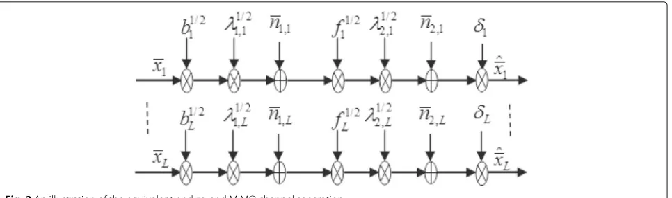
We consider a non-regenerative three-node two-hop MIMO relay system without the direct link between the source and the destination, as depicted in Fig. 1. The source, relay and destination haveM,KandNantennas, respectively. The half-duplex mode is assumed to be how the system operates. Each signal transmission from the source to the destination takes two time slots to complete. In the first time slot, the source node multiplies the signal vector x ∈ CM×1 by a source precoding matrix B ∈ CM×M. Here, the signal xcontains mutually cor-related data symbols with covariance matrix E(xxH) = Rx = x known to the three terminals sincexhas been arisen from encoding operations on the baseband signals [7]. The matrix x 0 denotes a correlation matrix with unit elements on its diagonal. The source precod-ing matrixBhas the power constraint tr(BRxBH) ≤ p1, wherep1is the allowed maximum transmit power at the source. Then, the resulting signal is transmitted to the relay node through the source-relay channelH1∈CM×K. The received signal at the relayy1 ∈ CK×1 is given by y1=H1Bx+n1, wheren1∈CK×1is the colored Gaussian noise vector at the relay with zero-mean and covariance matrix En1nH1
= Rn1 = σ12n1, and n1 0 is a correlation matrix with tr(n1)=K.
In the second time slot, at the relay, the received signal y1 is multiplied by a relay precoding matrix F ∈ CK×K satisfying the power constraint trFH1BRxBHHH1 +Rn1
FH
≤ p2, where p2 is the allowed maximum transmit power at the relay. After that, the resulting signalFy1is forwarded to the destina-tion through the relay-destinadestina-tion channel H2∈CK×N. Therefore, the received signal at the destinationy∈CN×1is
y=H2Fy1+n2=H2FH1Bx+H2Fn1+n2, (1)
where n2 ∈ CN×1is the colored Gaussian noise vector at the destination with zero-mean and covariance matrix E(n2nH2) = Rn2 = σ22n2, and n2 0 is a corre-lation matrix with tr(n2) = N. The channel matrices H1,H2 are generated base on Kronecker model [34] as Hi = 1i/2Hw,i1i/2,i = 1, 2, where the elements ofHw,i are i.i.d. zero-mean and unit-variance circularly symmet-ric complex Gaussian random variables andiandiare positive definite transmit and receive covariance matrices ofHi, and thereby,Hi∼CN(0,i⊗i).
We assume that rank
BR 1 2 x
= rank
FR 1 2 n1
= L
and L ≤ min(r1,r2), r1 = rank
R− 1 2 n1 H1
, r2 =
rank
R− 1 2 n2 H2
such that at most L independent
Fig. 1A non-regenerative three-node two-hop MIMO relay system
knowRn1 andRn2. An interesting example that relates to how to obtain these noise covariance matrices is given in [26] where the problem of designing the relay precoder in a three-node relay system in the presence of some interfer-ers near the destination by using the covariance informa-tion of the interferers-destinainforma-tion channels is addressed. Specifically, the received signal at the destination isy = H2FH1x+H2Fnw,1+Jj=1HIjxIj+nw,2, wherenw,1,nw,2
are the relay and destination white Gaussian noise vec-tors with covariance matrices Rnw,1 = σ12IK, Rnw,2 = σ2
2IN. It is assumed that the destination knows covari-ance matricesIj of the interferers-destination channels
HIj = Hw,j
1/2
Ij by the training signals that are friendly
shared by the interferersIj, and then the relay also knows Ij by feedback from the destination. It is valid to
equiv-alently view n2 Jj=1HIjxIj + nw,2 as the colored
noise vector at the destination. The destination can easily compute the destination-colored noise covariance matrix
Rn2 = E
n2nH2
by the covariance matrices Ij and
Rnw,2. The relay has Rn2 by feedback from the destina-tion. The source also hasRn2 by feedback from the relay. In a similar situation to the destination where the relay lies near some interferers such that y = H2FH1x + H2FJj=1H
Ijx
Ij+nw,1
+J
j=1HIjxIj +nw,2, the relay
can also have the covariance matrixRn1 =E
n1nH1
of the relay colored noisen1
J
j=1H
Ijx
Ij+nw,1by covariance
matrices of the interferers-relay channels andRnw,1. Then, Rn1 is fed back to the source, and fed forward to the des-tination by the relay. In other words, the three nodes all knowRn1besidesRn2. BesidesRx,Rn1, andRn2, the desti-nation is also assumed to haveH2FH1Bthrough a channel estimation method (e.g., [35–37]). The instantaneous MI between the source and the destination [31] is given by
I(B,F)= 1 2log2
IM+R
H
2
x BHHH1FHHH2
×H2FRn1FHHH2 +Rn2
−1
H2FH1BR 1 2 x
, (2)
where a factor 1/2 is due to the transmission duration of two time slots.
With the use of the linear MMSE equalizer [38]
G=RxBHHH1FHHH2
H2FH1BRxBHHH1FHHH2
+H2FRn1F HHH
2 +Rn2
−1 (3)
at the destination for signal detection as xˆ = Gy, the source-destination MI has an interesting relation with the MSE matrixME(xˆ−x)(xˆ−x)Hby [2]:
I(B,F)= −1
2log2|M|, (4)
where
M=
IM+R
H
2
x BHHH1FHHH2
×H2FRn1FHHH2 +Rn2
−1
H2FH1BR 1 2 x
−1 .
(5)
3 Joint source and relay precoding with the full CSIT
3.1 Optimal structures for source and relay precoders In this section, we assume that the source and the relay haveH1,H2, Rx, Rn1, andRn2 (the full CSIT). In prac-tice, the relay can estimateH1by the training signals sent from the source, and the destination can estimateH2by the training signals sent from the relay. The relay hasH2 by feedback from the destination, and the source hasH1 andH2by feedback from the relay. Note that feedbacking H2from the destination to the source is unusual due to the poor condition of the source-destination direct link [39], which is also assumed in this paper. With the full CSIT, we jointly designBandFto maximizeI(B,F)under the source and relay power constraints. This design issue can be formulated as:
max
Let us define the following singular value decomposi-tions (SVDs): and2are diagonal matrices of non-negative eigenvalues in descending order. In order to attain a maximum MI in Problem (6),BandFshould are optimally structured as:
B=V1 of non-negative entries with up toLpositive elements.
ProofApplying the matrix inversion lemma [40](A+
BCD)−1 = A−1 − A−1B(DA−1B + C−1)−1DA−1
Let us define ˜
Min (11) is rewritten more compactly as
M=IM− ˜HH1H˜H2
Let us define the eigenvalue decompositions (EDs) as ˜
1,H˜2 are the corresponding diagonal matrices of eigenvalues in descending order.
After some manipulations, we get
˜ to find that they do not affect the source and relay power constraints. After substituting (12) and (13) into (14) and performing some manipulations,Mbecomes
M = IM−XH1
Next, we consider the following properties:
For any Hermitian matrixAwith main diagonal vector
d(A)and eigenvalue vectorλ(A), thend(A)≺λ(A)[41]. Form N×Ncomplex matricesA1,A2,. . .,Amwith sin-gular values arranged in the same order as the product B= A1A2. . .Am, then the vector of singular values ofB is weakly majorized by the Schur (element-wise) product of the vectors of singular values of these complex values, that meansσ(B)≺wσ(A1)σ(A2). . .σ(Am)[41].
Let apply the above properties to, we have
d()≺λ()≺wd()˜ , (18)
where˜ = H1˜ (H1˜ +IM)−1H2˜ (H2˜ +IM)−1. Since −log2d(IM − )
is Schur-convex and increases with
d(), we get−log2d(IM−)
≤ −log2d(IM − ˜)
. This leads to
I≤ −1
Schur-convex and increasing function [41], and the maxi-mum of the MI is attained whenX1andX2are chosen as X1=IMandX2=UHH˜
1. Obviously, the MI is invariant in X1andX2.
Let us consider the source and relay transmit power constraints. From (7), (12), and (15), it is easy to compute
BR
The source transmit power can be rewritten as
trBRxBH
where the inequality exists because the fact that for any two N × N positive semidefinite matrices A and Bhaving the corresponding eigenvaluesλi(A)andλi(B) in the descending order, it follows that tr(AB) ≥
N
i λi(A)λN+1−i(B).
Obviously, in (19), the source transmit power is inde-pendent ofX1, and the minimum of the source power is achieved whenUH˜
H1 = U1. Besides, because we also have X1=IMas proved above,Bcan be obtained as
By setting 1
Similarly, from (8), (13), and (16),FR 1
The relay transmit power can be rewritten as
tr
It can be observed thatX2does not impact on the relay transmit power. Similar to (19), the equality in (20) holds whenUHH˜
2 =U2. Besides, since we also haveX2=U H
˜ H1as proved above,Fcan be calculated as
F=V2−12 optimalFas shown in (10).
One can see from (9) and (10) that the optimal set of B and F comes as a generalization of that for relay systems with i.i.d. channels, independent source signals, white noise of [4] to relay systems with spatially corre-lated channels, correcorre-lated input signals and colored noise. It is a development of the relay only precoding (ROP) with the sameF,Gas our design, butB= √p1/MIM of [28, 29]. Like the exiting designs with the full CSIT (e.g., [1–6, 8]), these optimal structures ofBandFare indepen-dent of the type of channel fading.Bperforms whitening the source signal streams, then loads the source power and beam-forms the obtained parallel signal streams across the eigenvectorsV1, whileFperforms whitening the relay colored noise, then loads the relay power across the eigen-vectorsUH1 andV2. By this way, the equivalent end-to-end MIMO channel in the presence of B, F, andGis sepa-rated into at mostLindependent subchannels (or eigen-modes) as illustrated in Fig. 2. This implies that there is no longer interference among the signal streams, which enhances the system capacity. This channel separation is mathematically expressed by
ˆ
is the diagonal matrix containing the
Fig. 2An illustration of the equivalent end-to-end MIMO channel separation
Setv (v1,. . .,vL)T andvl = (λ1,lbl+1)fl. Problem (22) can be rewritten as:
max
b,v≥0 I(b,v)= 1 2
L
l=1 log2
1+λ1,lbl+λ1,lblλ2,lvl+λ2,lvl 1+λ1,lbl+λ2,lvl
s.t. L
l=1
bl≤p1 and L
l=1 vl≤p2.
(23)
Once vl is found, fl can be easily computed as fl =
vl/(λ1,lbl + 1). An optimal solution to Problem (23) is impossible to obtain, since this problem is still non-concave inbandv. However, in the next two Sections 3.2 and 3.3, we design an iterative algorithm and a simplified algorithm to findbandv.
3.2 Iterative power allocation algorithm
In this section, we develop a numerical method based on alternating technique [3, 4, 8] to identifyb andv. It is important to find thatb andvbehave symmetrically in (23). Hence, if eitherborvis kept unchanged, Problem (23) turns to a standard concave optimization problem. Specifically, whenbis fixed, it collapses to the problem of optimizingvgiven by
max
v≥0 I(v)= 1 2
L
l=1 log2
1+λ1,lbl+λ1,lblλ2,lvl+λ2,lvl 1+λ1,lbl+λ2,lvl
(24)
s.t. L
l=1
vl≤p2. (25)
For the obtainedv, it reduces to the problem of optimiz-ingbgiven by
max
b≥0 I(b)= 1 2
L
l=1 log2
1+λ1,lbl+λ1,lblλ2,lvl+λ2,lvl 1+λ1,lbl+λ2,lvl
(26)
s.t. L
l=1
bl≤p1. (27)
We present how to obtainvfrom Problems (24)–(25). Let us consider the function
f(vl)=log2
1+λ1,lbl+λ1,lblλ2,lvl+λ2,lvl 1+λ1,lbl+λ2,lvl
.
Since it has the second derivative
d2f(v l) dv2l = −
λ2 2,l 2 ln 2
1
(1+λ2,lvl)2−
1
(1+λ1,lbl+λ2,lvl)2
≤0,
it is concave on 0 ≤ vl ≤ p2. It follows that the objec-tive functionI(v)= 12Ll=1log2f(vl)
is also concave on the same range ofvl. In addition, the constraint functions are clearly convex. Hence, Problems (24)–(25) is a stan-dard concave optimization problem [42] and its optimum solutionvcan be found via Lagrange method as follows.
Let introduce the Lagrange function as
L=I(v)+ν
L
l=1
vl−p2
− L
l=1 γlvl.
The concave functionI(v)achieves its global maximum when the Karush-Kuhn-Tucker (KKT) conditions [42], the necessary and sufficient conditions, as listed below, are satisfied:
−vl ≤0, γl≥0 and γlvl=0, (28)
ν≥0, ν
L
l=1
vl−p2
∂L ∂vl =
λ2,l 2 ln 2
1 1+λ2,lvl −
1 1+λ1,lbl+λ2,lvl
+ν−γl =0. (30)
Solving the system of Eqs. (28)–(30) yields the optimum water-fillingvas
vl=
⎡
⎣λ1,l
2λ2,lbl
2
+λ1,l λ2,l
blμv− λ1,l 2λ2,lbl−
1 λ2,l
⎤ ⎦
+
,
(31)
where the Lagrange multiplierμv1/νln 2 meets
L
l=1 ⎡
⎣ λ1,l
2λ2,l
bl
2
+λ1,l λ2,l
blμv−2λ2,λ1,l l
bl− 1
λ2,l
⎤ ⎦
+
=p2.
(32)
Since Problems (26)–(27) has the same form as Prob-lems (24)–(25), its optimal water-filling solutionbcan be inferred as:
bl=
⎡
⎣ λ2,l
2λ1,l
vl
2
+λ2,l λ1,l
vlμb−2λ1,λ2,l l
vl− 1 λ1,l
⎤ ⎦
+
,
(33)
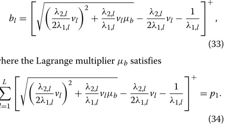
where the Lagrange multiplierμbsatisfies
L
l=1 ⎡
⎣ λ2,l
2λ1,l
vl
2
+λ2,l λ1,l
vlμb− λ2,l
2λ1,l
vl− 1
λ1,l
⎤ ⎦
+
=p1.
(34)
It is intuitively from (31) and (33) that F loads more power to the weaker eigenmodes of relay-destination link λ2,lthan the modified eigenmodes of the source-relay link
blλ1,l and less power to the stronger eigenmodes of the relay-destination linkλ2,l than the modified eigenmodes of the source-relay linkblλ1,l, whileBloads more power to the weaker eigenmodes of the source-relay link λ1,l than the modified eigenmodes of the relay-destination linkvlλ2,l and less power to the stronger eigenmodes of the source-relay linkλ1,lthan the modified eigenmodes of the relay-destination linkvlλ2,l. Here, the goal is to get as many optimal patterns of pairingblλ1,lwithvlλ2,las possi-ble to further enhance system capacity. This coordination of BandFis repeated until the achievement of desired system capacity. This iterative procedure is summarized briefly by Table 1. The computational complexity of the iterative design with the full CSIT is contributed by per-forming two SVDs in (7) and (8) with 2×O(L3)operations in which we takeL= N= M=Kfor simplicity, finding rootsvandbin (31) and (33) with 2×O(L)operations and searching the optimal patterns of pairingblλ1,l with
vlλ2,lwith 2×O(L!)operations. Hence, there are a total
Table 1An iterative algorithm to derivebandv
Compute1,2using (7) and (8)
Initializeb= p1
MIMsatisfying (27) Repeat
1) For a givenb, findvusing (31) and (32). ComputeI(b,v)(old).
2) For the obtainedv, findbusing (33) and (34). ComputeI(b,v)(new).
UntilI(b,v)(new)−I(b,v)(old)≤. Here >0 denotes a desired accuracy.
of 2×O(L3)+N ×(2×O(L)+2×O(L!))operations whereN represents the number of iterations required to complete this iterative design.
In the design process, besides the covariance matrices Rx,Rn1, andRn2, the relay needs to have the estimated CSI H1 and the destination-relay feedback CSIH2, and the source needs to have the relay-source feedback CSIH1 andH2. With each set of such the full CSIT, for fixedb, the relay computesv, and then feeds back it to the source. The source updatesbwith the receivedv, and then feeds forward the updatedb to the relay. To obtain an output ofvandb, this updating is repeated alternatively between the relay and the source untilI(b,v)converges a desired value. Due to computational burden of such the iterative procedure, its output ofvandb, thus the precodersBand Fmay be outdated to the current propagation condition. In practical wireless communications systems, to effi-ciently mitigate the overhead and the design complexity, codebook and limited feedback schemes are often uti-lized. The idea behind these techniques is that the receiver first would quantize the estimated CSI, and feedback the resulting index to the transmitter. The transmitter then picks the desired precoder from a codebook which is a set of precoders designed offline beforehand by using various CSIT sets [39].
3.3 Simplified power allocation algorithm
In this section, we develop a simplified algorithm that allows to load source and relay power separately. First, let consider the inequality:
(1+x)(1+y)
1+x+y ≤(1+x)(1+y), (35)
where x and y are two non-negative scalars. Applying inequality (35) to the objective function of Problem (23) leads to its upper bound that is equal to
1 2
L
l=1
log21+λ1,lbl+1
2 L
l=1
In (23), let replace the objective function with its upper bound. Consequently, Problem (23) can be split to two concave optimization problems as:
max
The corresponding optimal water-filling solutionsvand bto Problems (37) and (38) are, respectively, given by [20]:
vl=
It is intuitively from (39) and (40) that F loads more power to the weaker eigenmodes of the relay-destination linkλ2,land less power to the strongerλ2,l, whileBloads more power to the weaker eigenmodes of the source-relay linkλ1,l and less power to the strongerλ1,l. In the design process, the relay needs to haveRx,Rn1,Rn2,H1, andH2, while the source needs to haveRx,Rn1, andH1. With each set of such the full CSIT, the relay computesvand feeds back it to the source, and then the source calculatesb with the received v. Because there is no need for feed-backingRn2 andH2to the source, the simplified design with the full CSIT allows to save a large signaling overhead compared to the iterative counterpart. In terms of the computational complexity, this simplified design requires 2×(O(L3)+O(L)+O(L!))operations to accomplish, thus it is much simpler than the iterative counterpart. Because of the simplicity of separately calculatingvandb, the sim-plified scheme may give lower capacity than the iterative scheme. Nevertheless, we can expect that its capacity per-formance is comparable to the perper-formance of the the iterative counterpart, especially at the medium-to-high SNRs. This is mainly due to the fact that in inequality (35), whenx,y → ∞, then 1+x+y (1+x)(1+y), or
equivalently, whenb,v → ∞(i.e.,p1/σ12,p2/σ22 → ∞), thenI(b,v)approaches to its upper bound. Interestingly, this simplified design can be also extended to the case of multi-hop systems, as presented below.
Let extend inequality (35) toZ≥2 non-negative scalars
x1,. . .,xZ. The obtained inequality is
By this inequality, an upper bound MI of aZ-hop system can be derived as
1
Similar to the two-hop system case, the entriesblof the diagonal matrixbof the source precoding matrix
B=V1
can be found by solving the corresponding optimization problems given by:
max 1 Solving Problems (43) and (44) yields [20]
bl=
This shows the flexibility of our proposed design methods. Theorem 1 below concludes the main results on the joint design of source and relay precoders with the full CSIT.
Theorem 1The instantaneous mutual information
I(B,F)attains its maximum under the power constraints
tr(BRxBH) ≤ p1andtr
V2 are unitary matrices of R
−1
ces of non-negative entries which can be determined alter-nately by the iterative algorithm (Section 3.2) or separately by the simplified algorithm (Section 3.3).
4 Joint source and relay precoding with partial CSIT
4.1 Suboptimal structures for source and relay precoders In Section 3, we obtained the precoder designs with the full CSIT. However, it is too hard for the relay and the source to obtain H2 in the situation when the desti-nation moves rapidly. This is basically because a large amount of signalling overhead is needed for feedbacking H2, while the feedback channels in practical wireless sys-tems are commonly rate-limited. For these reasons, in this section, we assume that the source and the relay have Rx,Rn1,Rn2,H1, and only covariance information2and 2 ofH2 (the partial CSIT). With the partial CSIT, we jointly design BandF to maximize EH2I(B,F) under the source and relay transmit power constraints. However, it is intractable to exactly compute EH2
I(B,F)because taking the expectation with respect to unknownsBandF is needed. Here, an alternative solution proposed is to use its an upper bound, which is derived below.
Applying the matrix inversion lemma to (5) gives
M=W−1+W−1 inequality [44] and the property which states that for any matrix H with the distribution H ∼ CN(0, ⊗ ), is found as
EH2(I(B,F))≤ −1 The design problem now is relaxed to
max
Let us define the following SVDs:
R− andθare diagonal matrices of non-negative eigenvalues in descending order. In order to achieve a maximum of
where (bp) and f(p) are M× M and K ×K diagonal matrices of non-negative entries with up to L positive elements.
ProofLet us define
˜
Again, by the matrix inversion lemma, ML in (46) is simplified to
ML=IM− ˜HH1HHθ(Hθ(H˜1H˜H1+IK)HHθ +IN)−1HθH˜1. (54)
Clearly,MLhas the same form asMin (14). Therefore, the proof part of the optimal source and relay precoder structures with the full CSIT in (9) and (10) presented in Part 3 can be used for the derivation of those with the partial CSIT in (50) and (51).
In [5, 6], the ROP schemes were obtained using the partial CSIT for two-hop relay systems with only transmit-sided spatially correlated channels, white noises, and independent source symbols. These schemes are actually included in our proposed joint precoding with the partial-CSIT as special cases. In fact, by substituingRx = IM, Rn1 = σn12IK, Rn2 = σn22IN, 2 = IN into (50) and (51), the source and relay precoding reduce to the ROP in [5, 6]. Since the relay eigen-beamer directionsVθdoes not match the relay-destination subchannel directionsV2, the obtained partial-CSIT precoders are clearly subopti-mal compared to the full-CSIT precoders. Therefore, the system capacity enhancement much relies on how to allo-cate power across the source and relay antennas. This task is equivalent to solving a problem of optimizing(bp)and (p) can be rewritten as:
max (56) is impossible due to its non-concavity in b(p) and v(p). Therefore, we propose to deal with this problem by an iterative algorithm in Section 4.2 and by a simplified algorithm in Section 4.3.
4.2 Iterative power allocation algorithm
Interestingly,b(p) andv(p)are symmetrical each other in (56). Therefore, if eitherb(p)orv(p)is kept fixed, Problem (56) becomes a standard concave optimization problem. Specifically, for a givenb(p), it collapses to the problem of optimizingv(p)given by
Similarly to Section 3.2, an iterative algorithm for find-ingb(p)andv(p)alternatively is also developed, as shown in Table 2.
Table 2An iterative algorithm to deriveb(p)andv(p)
Compute1,θusing (7) and (49) Initializeb(p)= p1
MIMsatisfying (60) Repeat
1) Findv(p)(i.e., the solution to problem (57)) for the fixedb(p)using
vl(p)= λ1,l whereμv>0 satisfies
L
2) Findb(p)(i.e., the solution to problem (59)) with the obtainedv(p)using
b(p)l = a desired accuracy.
each iteration. As a result, the overall system capacity increases after the algorithm terminates. The complexity of the iterative precoder design with the partial CSIT is nearly the same as the complexity of the iterative precoder design with the full CSIT, with a total of 2×O(L3)+N× (2×O(L)+2× O(L!))operations. In the design pro-cess, besidesRx,Rn1,Rn2, andH1, the source and the relay only need to have covariance information2 and2of H2. Since these covariance matrices change much slower compared to their channel realizationH2, a large mount of signaling overhead and the design complexity required are significantly saved compared to the iterative design with the full CSIT. These benefits thus allow to broaden the applicability of the iterative design with the partial CSIT in practical communications systems, especially when it is realized by codebook and limited feedback techniques [39] that we discussed in Section 3.2.
4.3 Simplified power allocation algorithm
In this section, to reduce the computational complexity of the iterative algorithm in Section 4.2, we develop its simplified algorithm. By inequality (35), an upper bound of the objective function of Problem (56) can be derived equal to
In (56), let us replace the objective function with its upper bound. As a result, Problem (56) can be decoupled into two concave optimization problems given by:
max
Again, the optimal water-filling solutionsv(p)andb(p)to the respective problems (62) and (63) are given by [20]:
v(lp)=
It is obviously from (64) and (65) that F loads more power to the weaker eigenmodes of the transmit covari-ance matrix of the relay-destination link γ λθ,l and less power to the strongerγ λθ,l, whileBloads more power to the weaker eigenmodes of the source-relay link λ1,l and less power to the stronger λ1,l. The relay needs to have Rx,Rn1,Rn2,H1,2and2, while the source only need to haveRx,Rn1,H1. With each set of such the partial CSIT, the relay computesv(p) and feeds back it to the source, and then the source calculatesb(p)with the receivedv(p). Obviously, the simplified design with the partial CSIT requires less signaling overhead than the iterative design with the partial CSIT and the simplified design with the full CSIT. Besides, its computational complexity is the same as that of the simplified design with the full CSIT, and much less than that of the iterative design with the partial CSIT. Despite its simplicity, the simplified design with the partial CSIT works well, especially at high SNRs. This is mainly due to the fact that in inequality (35), when
x,y→ ∞, then 1+x+y(1+x)(1+y), or equivalently, when whenb(p),v(p)→ ∞(i.e.,p1/σ12,p2/σ22→ ∞), then
˙
Ierg(b(p),v(p))approaches to its upper bound.
Theorem 2 below summarizes the main results on jointly designing source and relay precoders with the partial CSIT.
Theorem 2The average mutual informationEH2I(B,
F) achieves its maximum under the power constraints
tr(BRxBH) ≤ p1 and tr
F(H1BRxBHHH1 +Rn1)FH
≤
V1
(p) b
1 2
R− 1 2
x andF = Vθ
(p)
f
1 2
UH1R− 1 2
n1 . Here,U1,
Uθ,V1andVθare unitary matrices ofR− 1 2
n1 H1=U1 1 2 1VH1
andγ12 1 2
2 = Uθ
1 2
θVHθ, and(bp)and
(p)
f are diagonal
matrices of non-negative entries which can be determined alternately by the iterative algorithm (Section 4.2) or sepa-rately by the simplified algorithm (Section 4.3).
5 Simulation results
In this section, the proposed iterative and simplified pre-coding designs with the full CSIT and with the partial CSIT are evaluated in terms of system capacity by numer-ical simulations. The considered relay system has the transmit and receive covariance matricesiandi,i = {1, 2}in the corresponding Toeplitz forms [6, 12] as
i(n,m)=rt|n−m|, n,m= {1,. . .,M}, i(n,m)=rr|n−m|, n,m= {1,. . .,K},
where correlation coefficientsrt, rr meet rt,rr ∈ (0, 1]. Like [2, 5, 6], the source powerp1 includes the source-relay path-loss, and the source-relay powerp2includes the relay-destination path-loss. SNR1 p1/σ12 is defined as the first-hop SNR, and SNR2 p2/σ12 as the second-hop SNR. The source, relay, and destination nodes all have four antennas (M= K =N =4). The correlation matrices of source signals, relay and destination noises are chosen as
x=
⎡ ⎢ ⎢ ⎣
1.0000 −0.5715 0.7742 −0.6025 −0.5715 1.0000 −0.6905 0.5062
0.7742 −0.6905 1.0000 −0.6387 −0.6025 0.5062 −0.6387 1.0000
⎤ ⎥ ⎥ ⎦,
n1 =
⎡ ⎢ ⎢ ⎣
1.0000 0.2637 −0.1939 0.3348 0.2637 1.0000 −0.1141 0.1194 −0.1939 −0.1141 1.0000 0.2085 0.3348 0.1194 0.2085 1.0000
⎤ ⎥ ⎥ ⎦,
n2 =
⎡ ⎢ ⎢ ⎣
1.0000 0.6709 −0.3419 0.5644 0.6709 1.0000 −0.6666 0.5062 −0.3419 −0.6666 1.0000 −0.4288
0.5644 0.5062 −0.4288 1.0000 ⎤ ⎥ ⎥ ⎦.
The noise correlation matrices are chosen randomly as long as the noises are colored enough but do not totally interfere the other channel factors. The first condition is to make sure that the noises will have a “colored” effect to the system, while the second one is to maintain the prac-tical meaning of the wireless model. The matrixn1 has the vector of eigenvalues [1.5000, 1.2000, 0.8000, 0.5000], n2 has the vector of eigenvalues [2.6000, 0.7000, 0.5000, 0.2000],x has the vector of eigenvalues [2.9000, 0.5000, 0.4000, 0.2000]. The Matlab command used to generate n1randomly is gallery(’randcorr’, [1.5000, 1.2000, 0.8000, 0.5000])1. Like previous references [28–31, 45–47], the colored noise vectorn1 ∼ CN(0,σ12n1)is generated as
n1 =
1 2
n1nw,1, wheren1w,1 ∼ CN(0,σ12IK)is the white
noise vector. The matrix 1 2
n1 plays a role as the digital filter, and it uniquely exists sincen1 is positive semidef-inite [19, 40].x,xandn2,n2are also generated by the same way asn1 andn1. Note that in [21–25], the covari-ance matrix of the relay colored noise is generated via a first order autoregressive filter as Rn1(i,j) = α1r1η|1i−j|, wherer1is a normalization factor to keep tr(Rn1)=α1K, andα1denotes the interference power from the neighbour interferers. In comparison with our colored noise simula-tion method,α1functions asσ12, whiler1η|1i−j| functions asn1(i,j).
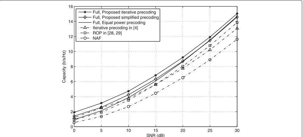
Figures 3 and 4 reveal the system capacity perfor-mance of the proposed iterative and simplified precoding designs with the full CSIT in Section 3. As pointed out in Section 3.3, the precoding in [30, 31] has the same precod-ing design result as the simplified precodprecod-ing, so its results are not illustrated in this section. The iterative precoding in [4], the ROP in [28, 29], the naive amplify-and-forward (NAF) scheme [4] havingB=!p1/tr(Rx)IMand
F=
p2
trH1BRxBHHH1 +Rn1
IK
are chosen as comparatives. Note that all the consid-ered schemes are based on the full CSIT. As discussed in Section 3.1, their precoder structures do not vary with an effect of the spatially correlated channel fading, and thus the spatial correlationsrt=rr =0.5 are chosen for all the involved channels.
0 5 10 15 20 25 30 0
2 4 6 8 10 12
Capacity (b/s/Hz)
SNR
1 (dB)
Full, Proposed iterative precoding Full, Proposed simplified precoding Full, Equal power precoding Iterative precoding in [4] ROP in [28, 29] NAF
Fig. 3A performance comparison of the precoding schemes with the full CSIT for SNR2=20dBandrt=rr=0.5
that the optimality in the precoder structures alone con-tributes a significant portion in the capacity enhancement. A well-designed water-filling power allocation adds fur-ther capacity, especially in the low SNR regime.
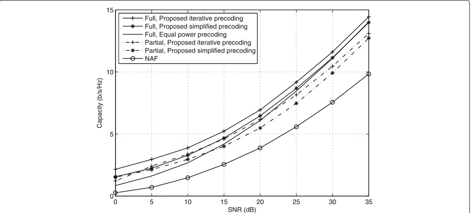
Besides the signal, relay and destination noise corre-lation matrices, the performance of the precoder struc-truces and the power allocation schemes is a function of the available CSIT types and quality of constituent channels: SNR1, SNR2 and the spatial correlations. This statement is shown in Figs. 5, 6, 7, and 8. These figures
demonstrate a number of performance comparisons among all the proposed precoding designs with the full CSIT as well as with the partial CSIT. As aforementioned in Section 4.1, the ROP schemes in [5, 6] designed for two-hop relay systems with transmit-sided spatially cor-related channels, white noises, independent symbols are included in the proposed partial-CSIT precoding designs. Clearly, there is no valuable information for the use of these schemes as the performance references. Hence, their behaviours are not shown in Figs. 5, 6, 7 and 8. Figure 5
0 5 10 15 20 25 30
0 2 4 6 8 10 12 14 16
Capacity (b/s/Hz)
SNR (dB) Full, Proposed iterative precoding Full, Proposed simplified precoding Full, Equal power precoding Iterative precoding in [4] ROP in [28, 29] NAF
0 5 10 15 20 25 30 0
2 4 6 8 10 12 14 16
Capacity (b/s/Hz)
SNR (dB) Full, Proposed iterative precoding Full, Proposed simplified precoding Full, Equal power precoding Partial, Proposed iterative precoding Partial, Proposed simplified precoding NAF
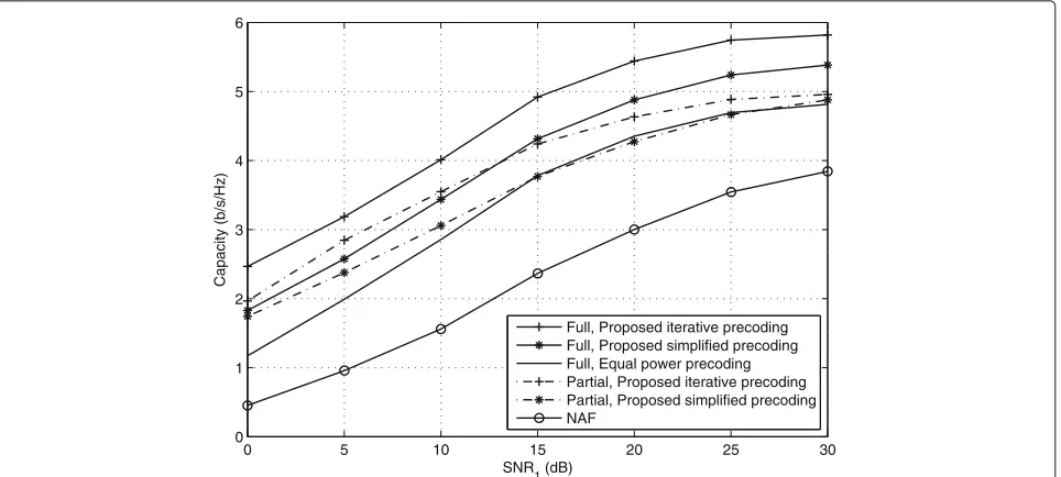
Fig. 5A performance comparison of the proposed precoding designs for SNR1=SNR2=SNR,rt=rr=0.3
shows the capacity of systems having SNR2 = SNR2 = SNR andrt = rr = 0.3, and Fig. 6 shows the capacity of systems having SNR2 = SNR2 = SNR and rt = 0.95,rr = 0.3. The correlation coefficent rt = 0.95 represents a strong correlation effect among the trans-mit antennas since the corresponding correlation matrix has the eigenvalues [3.7568, 0.1627, 0.0506, 0.0300] with the very large condition number 125.2267. It is clear to observe that when rt increases from 0.3 to 0.95, capac-ity gains of the proposed precoding designs over the NAF
scheme increase, and capacity gaps of the full CSIT based designs over the partial CSIT based designs decrease. The partial CSIT based designs provide higher capacity than the equal power precoding at low to medium SNRs. These higher capacity regions are even enlarged with increase in the transmit correlation.
How the schemes based on the partial CSIT behave for rt = 0.95,rr = 0.3 will be revealed more clearly in Figs. 7 and 8. Figure 7 plots the curves of capacity as a function of SNR1 and SNR2 = 12dB, and Fig. 8
0 5 10 15 20 25 30 35
0 5 10 15
Capacity (b/s/Hz)
SNR (dB) Full, Proposed iterative precoding Full, Proposed simplified precoding Full, Equal power precoding Partial, Proposed iterative precoding Partial, Proposed simplified precoding NAF
0 5 10 15 20 25 30 0
1 2 3 4 5 6
Capacity (b/s/Hz)
SNR
1 (dB)
Full, Proposed iterative precoding Full, Proposed simplified precoding Full, Equal power precoding Partial, Proposed iterative precoding Partial, Proposed simplified precoding NAF
Fig. 7A performance comparison of the proposed precoding designs for SNR2=12dB,rt=0.95,rr=0.3
shows the curves of capacity as a function of SNR2and SNR1=12dB. The results from these figures reveal there are more clearer extensions in the capacity gains of the precoding techniques to the NAF technique. Amongst the considered techniques, the iterative precoding tech-niques based on the full CSIT still provides the best capacity gain. Besides, the capacity gaps among all the precoding schemes also increase, especially for the ones based on the full CSIT. Figure 7 indicates that when
SNR2 = 12dBour both designs with the partial CSIT outperform the equal precoding, and more interestingly, the iterative design with the partial CSIT yields higher capacity than the simplified design with the full CSIT over the low-to-medium SNR1 range, with up to 15dB. Figure 8 indicates when SNR1 = 12dB, the iterative design with the partial CSIT gives the same performance as the simplified design with the full CSIT at low-to-medium SNR2 levels, but gives the higher performance
0 5 10 15 20 25 30 35
1 1.5 2 2.5 3 3.5 4 4.5 5 5.5
Capacity (b/s/Hz)
SNR
2 (dB)
Full, Proposed iterative precoding Full, Proposed simplified precoding Full, Equal power precoding Partial, Proposed iterative precoding Partial, Proposed simplified precoding NAF
than this scheme at higher SNR2 levels. While the sim-plified design with the partial CSIT not only extends the capacity gaps over the equal precoding but also cre-ates the capactiy curve closer to that of the simplified design with the full CSIT, especially at low and high SNR2levels.
These observations verify the effectiveness of the water-filling-typed power allocation strategies of the partial-CSIT-based designs, especially when the involved channels are in medium SNR environments and are strongly affected by the spatial correlation fading at the transmit sides, regardless of the mismatch between the relay eigen-beamer directions (Vθ) and the relay-destination subchannel directions (V2) as aforementioned in Section 4.1.
6 Conclusions
In summary, we developed the iterative and simplified methods of jointly designing of source and relay precoders with the full CSIT and those with partial CSIT for gen-eral correlated dual-hop MIMO relay systems without the direct link under the MMI criterion. These general systems have spatially correlated channels, mutually cor-related source signals and colored noises. We showed the optimal source and relay precoder obtained with the full CSIT and the destination equalizer altogether decouple the equivalent end-to-end MIMO channel into orthogo-nal SISO subchannels. We also successfully extended the simplified precoder design with the full CSIT to the multi-hop relay system case. Simulation results showed that the proposed joint precoder designs with the full CSIT pro-vide higher capacity than the existing designs. Also, the proposed joint precoder designs with the partial CSIT work well, especially when the channels are strongly cor-related at the transmit sides and at medium-to-high SNRs, while they require much lower computational complexity and less feedback overhead. In future work, we would consider the relay system case where the distance between the source and the destination is short enough for them to directly communicate each other, thus the direct link is taken into account. We would propose joint source and relay precoding schemes that exploit CSI of the compound relaying link and the direct link for the system capacity maximization.
Endnote
1With a given K ×1 vector x of non-negative
ele-ments summing to K, we always create a K × K
real symmetric positive semidefinite matrix, i.e., cor-relation matrix A as A = UHdiag(x)U, where U is a unitary matrix. Here, the correlation matrix A has unit elements on its main diagonal and eigenvalues given byx[41].
Competing interests
The authors declare that they have no competing interests.
Received: 2 February 2016 Accepted: 16 February 2017
References
1. X Tang, Y Hua, Optimal design of non-regenerative MIMO wireless relays. IEEE Trans. Wireless Commun.6(4), 1398–1407 (2007)
2. O Munoz, J Vidal, A Agustin, Linear transceiver design in nonregenerative relays with channel sate information. IEEE Trans. Signal Process.55(6), 2593–2604 (2007)
3. R Mo, YH Chew, Precoder design for non-regenerative MIMO relay systems. IEEE Trans. Wireless Commun.8(10), 5041–5049 (2009) 4. Z Fang, Y Hua, JC Koshy, inFourth IEEE Workshop on Sensor Array
Multi-channel Signal Processing. Joint source and relay optimization for a non-regenerative MIMO relay, (Waltham, 2006), pp. 239–243
5. C Jeong, H-M Kim, Precoder design of non-regenerative relays with covariance feedback. IEEE Commun. Lett.13(12), 920–922 (2009) 6. C Jeong, B Seo, SR Lee, H-M Kim, I-M Kim, Relay precoding for
non-regenerative MIMO relay systems with partial CSI feedback. IEEE Trans. Wireless Commun.11(5), 1698–1711 (2012)
7. D Gesbert, M Shafi, A N, From theory to practice: an overview of MIMO space-time coded wireless systems. IEEE J. Selected Areas Commun. 3(21), 281–302 (2003)
8. Y Rong, X Tang, Y Hua, A unified framework for optimizing linear nonregenerative multicarrier MIMO relay communication systems. IEEE Trans. Signal Process.57(12), 4837–4851 (2009)
9. D-H Kim, HM Kim, in21st Annual IEEE International Symposium on Personal, Indoor and Mobile Radio Communications. MMSE precoder design for a non-regenerative MIMO relay with covariance feedback, (2010), pp. 461–464. doi:10.1109/PIMRC.2010.5671893
10. L Gopal, Y Rong, Z Zang, inThe 17th Asia Pacific Conference on Communications. Joint MMSE transceiver design in non-regenerative MIMO relay systems with covariance feedback, (2011), pp. 290–294. doi:10.1109/APCC.2011.6152821
11. L Gopal, Y Rong, Z Zang, in2013 IEEE 77th Vehicular Technology Conference (VTC Spring). MMSE based transceiver design for MIMO relay systems with mean and covariance feedback, (2013), pp. 1–5.
doi:10.1109/VTCSpring.2013.6692635
12. N Fawaz, K Zarifi, M Debbah, D Gesbert, Asymptotic capacity and optimal precoding in MIMO multi-hop relay networks. IEEE Trans. Inform. Theory. 57(4), 2050–2069 (2011)
13. C Xing, S Ma, Y-C Wu, Robust joint design of linear relay precoder and destination equalizer for dual-hop amplify-and-forward MIMO relay systems. IEEE Trans. Signal Process.58(4), 2273–2283 (2010)
14. B Zhang, Z He, K Niu, L Zhang, Robust linear beamforming for MIMO relay broadcast channel with limited feedback. IEEE Signal Process. Lett.17(2), 209–212 (2010)
15. W Xu, X Dong, W-S Lu, MIMO relaying broadcast channels with linear precoding and quantized channel state information feedback. IEEE Trans. Signal Process.58(10), 5233–5245 (2010)
16. Y Rong, Robust design for linear non-regenerative MIMO relays with imperfect channel state information. IEEE Trans. Signal Process.59(5), 2455–2460 (2011). doi:10.1109/TSP.2011.2113376
17. Z Wang, W Chen, J Li, Efficient beamforming for MIMO relaying broadcast channel with imperfect channel estimation. IEEE Trans. Veh. Technol. 61(1), 419–426 (2012)
18. Y Cai, RC de Lamare, L-L Yang, M Zhao, Robust mmse precoding based on switched relaying and side information for multiuser MIMO relay systems. IEEE Trans. Veh. Technol.64(12), 45677–5687 (2015)
19. C Chien,Digital Radio Systems on A Chip: A System Approach. (Kluwer Academic, 2001)
20. A Scaglione, GB Giannkis, S Barbarossa, Redundant filterbank precoders and equalizers. Part I: unification and optimal designs. IEEE Trans. Signal Process.47(7), 1988–2006 (1999)
21. M Biguesh, S Gazor, MH Shariat, Optimal training sequence for MIMO wireless systems in colored environments. IEEE Trans. Sig. Process.57(8), 3144–3153 (2009)
23. R Wang, M Tao, H Mehrpouyan, Y Hua, Channel estimation and optimal training design for correlated MIMO two-way relay systems in colored environment (2014). http://arxiv.org/abs/1407.5161
24. R Wang, M Tao, H Mehrpouyan, Y Hua, Channel estimation and optimal training design for correlated MIMO two-way relay systems in colored environment. IEEE Trans. Wire. Commun.14(5), 2684–2699 (2015) 25. R Wang, H Mehrpouyan, M Tao, Y Hua, inIEEE Glob. Commun. Conf. Optimal
training design and individual channel estimation for MIMO two-way relay systems in colored environment, (Austin, 2014), pp. 3561–3566 26. C Jeong, HM Kim, HK Song, IM Kim, Relay precoding for non-regenerative
MIMO relay systems with partial CSI in the presence of interferers. IEEE Trans. Wireless Commun.11(4), 1521–1531 (2012).
doi:10.1109/TWC.2012.020812.111246
27. NN Tran, HD Tuan, HH Nguyen, Training signal and precoder designs for OFDM under colored noise. IEEE Trans. Vehic. Technol.57(6), 3911–3917 (2008)
28. NA Vinh, NN Tran, NH Phuong, Optimal precoding design for non-regenerative dual-hop correlated relaying MIMO. Electron. Lett. 51(20), 1613–1615 (2015)
29. NA Vinh, NN Tran, NH Phuong, DL Khoa, in2015 NAFOSTED Conference on Information and Computer Science. Optimally non-regenerative relaying for general dual-hop correlated MIMO channels, (Hochiminh, 2015), pp. 300–304
30. NN Tran, S Ci, in2010 IEEE Global Telecommunications Conference (GLOBECOM 2010). Asymptotic capacity and precoding design for correlated multi-hop MIMO channels, (Miami, 2010), pp. 1–5 31. NN Tran, S Ci, HX Nguyen, CMI analysis and precoding designs for
correlated multi-hop MIMO channels. EURASIP Journal on Wireless Communications and Networking, (127) (2015)
32. M Vu, A Paulraj, MIMO wireless linear precoding using CSIT to improve link performance. IEEE Signal Process. Mag.87, 86–105 (2007)
33. AK Gupta, DK Nagar,Matrix Variate Distributions. (Chapman and Hall/CRC, USA, 1999)
34. D-S Shiu, GJ Foschini, M J.Gans, J M.Kahn, Fading correlation and its effect on the capacity of multielement antenna systems. IEEE Trans. Commun. 48(3), 502–513 (2000)
35. NN Tran, HH Nguyen, HD Tuan, DE Dodds, Training designs for amplify-and-forward relaying with spatially correlated antennas. IEEE Trans. Vehic. Technol.61, 2864–2870 (2012)
36. S Sun, Y Jing, Channel training design in amplify-and-forward MIMO relay networks. IEEE Trans. Wire. Commun.10(10), 920–922 (2011)
37. J-S Sheu, J-K Lain, W-H Wang, On channel estimation of orthogonal frequencydivision multiplexing amplify-and-forward cooperative relaying systems. IET Commun.7(4), 325–334 (2013)
38. SM Kay,Fundamentals of Statistical Signal Processing, Volume 1: Estimation Theory. (Prentice Hall, New Jersey, 1993)
39. DJ Love, RW Heath, VKN Lau, D Gesbert, BD Rao, M Andrews, An overview of limited feedback in wireless communication systems. IEEE J. Selected Areas Commun.26(8), 1341–1365 (2008). doi:10.1109/JSAC.2008.081002 40. KB Petersen, MS Pedersen,The Matrix Cookbook. (Technical University of
Denmark, 2012)
41. AW Marshall, I Olkin, BC Arnold,Inequalities: Theory of Majorization and Its Applications - Second Edition. (Springer, New York, 2011)
42. S Boyd, L Vandenberghe,Convex Optimization. (Cambridge University Press, New York, 2004)
43. E Jorswieck, H Boche,Majorization and Matrix-Monotone Functions in Wireless Communications. (Hanover, MA: Now Publishers, 2007) 44. RA Horn, CR Johnson,Matrix Analysis. (Cambridge University Press,
New York, 1985)
45. NN Tran, HD Tuan, HH Nguyen, Training signal and precoder designs for OFDM under colored noise. IEEE Trans. Veh. Techno.57(6), 3911–3917 (2008)
46. NN Tran, HX Nguyen, Optimal SP training for spatially correlated MIMO channels under coloured noises. Electron. Lett.51, 247–249 (2015) 47. G Panci, S Colonnese, P Campisi, G Scarano, Blind equalization for
correlated input symbols: a bussgang approach. IEEE Trans. Signal Process.53(5), 1860–1869 (2005)
Submit your manuscript to a
journal and benefi t from:
7Convenient online submission
7Rigorous peer review
7Immediate publication on acceptance
7Open access: articles freely available online 7High visibility within the fi eld
7Retaining the copyright to your article