An improved regularization method for estimating near real-time systematic
errors suitable for medium-long GPS baseline solutions
Xiaowen Luo1,2, Jikun Ou1, Yunbin Yuan1, Jinyao Gao2, Xianglong Jin2, Kefei Zhang3, and Huajun Xu1
1Institute of Geodesy and Geophysics, Chinese Academy of Sciences, Wuhan 430077, China 2Key Laboratory of Submarine Geosciences, SOA, Hangzhou 310012, China 3School of Mathematical and Geospatial Sciences, RMIT University, Australia
(Received June 7, 2007; Revised April 14, 2008; Accepted April 14, 2008; Online published September 8, 2008)
It is well known that the key problem associated with network-based real-time kinematic (RTK) positioning is the estimation of systematic errors of GPS observations, such as residual ionospheric delays, tropospheric delays, and orbit errors, particularly for medium-long baselines. Existing methods dealing with these systematic errors are either not applicable for making estimations in real-time or require additional observations in the computation. In both cases, the result is a difficulty in performing rapid positioning. We have developed a new strategy for estimating the systematic errors for near real-time applications. In this approach, only two epochs of observations are used each time to estimate the parameters. In order to overcome severe ill-conditioned problems of the normal equation, the Tikhonov regularization method is used. We suggest that the regularized matrix be constructed by combining the a priori information of the known coordinates of the reference stations, followed by the determination of the corresponding regularized parameter. A series of systematic errors estimation can be obtained using a session of GPS observations, and the new process can assist in resolving the integer ambiguities of medium-long baselines and in constructing the virtual observations for the virtual reference station. A number of tests using three medium- to long-range baselines (from tens of kilometers to longer than 1000 kilometers) are used to validate the new approach. Test results indicate that the coordinates of three baseline lengths derived are in the order of several centimeters after the systematical errors are successfully removed. Our results demonstrate that the proposed method can effectively estimate systematic errors in the near real-time for medium-long GPS baseline solutions.
Key words:Medium-long baselines, systematic errors, GPS network RTK positioning, ill-conditioned equation, Tikhonov regularization.
1.
Introduction
It is well-known that the conventional RTK GPS system has many practical limitations. One of these is that the rover station has to be located in the vicinity of a base station (usually less than 10–20 km). As a result, there are only a few redundant observations, which leads to the difficulty of checking gross errors and less positioning reliability (Gaoet al., 1997; Chenet al., 2001; Zhanget al., 2006). The recent development of the multi-reference stations GPS network technology (i.e. network RTK) enables high-precision RTK positioning to be realized for medium-long baselines (typ-ically between 30–150 km), and this technology has been successfully implemented in many experiments (e.g. Chen
et al., 2000; Lachapelleet al., 2000; Odijket al., 2000; Vol-lathet al., 2000; Raquet and Lachapelle, 2001; Landauet al., 2003; Vollathet al., 2002; Huet al., 2003; Rizos and Han, 2003; Alves, 2004).
The core component of this technology is to rapidly and accurately fix the integer ambiguities of the baselines among the reference stations in a Continuously Operating Reference Station (CORS) network in real-time. However,
Copyright cThe Society of Geomagnetism and Earth, Planetary and Space Sci-ences (SGEPSS); The Seismological Society of Japan; The Volcanological Society of Japan; The Geodetic Society of Japan; The Japanese Society for Planetary Sci-ences; TERRAPUB.
the success rate of integer ambiguity resolution is affected by the residual systematic errors in the baselines. Since the characteristics of the systematic errors are continual as well as incidental, it is difficult to describe them using a unified and deterministic model (Yang, 1999; Zhouet al., 1999). Current methods for estimating systematic errors in network RTK can be divided into two steps: (1) reso-lution of the double-differenced (DD) integer ambiguities between the baselines and (2) substitution into theDD ob-servation equations to compute the systematic errors of the corresponding baseline (Huet al., 2003). Although a great deal of published research has focused on the resolution of the integer ambiguity (e.g. Sunet al., 1999; Daiet al., 2003; Chenet al., 2004), additional observation data are usually involved in the computation. The characteristics of system-atic errors of the medium-long baseline network have also been studied (e.g. Han and Rizos, 1996; Fotopoulos and Cannon, 2000). The results of such studies indicate that the systematic errors are correlated with time for the obser-vations of two adjacent epochs. They may, therefore, be expressed as a function of time and be computed using a Kalman filtering technique (Daiet al., 2003). However, es-timating the systematic errors rapidly using actual observa-tions is still a challenge in the study of systematic errors of the medium-long baseline network RTK, especially when
estimating the systematic errors in near real time is dis-cussed in Section 3. Experiment results are analyzed in Section 4, and some conclusions are drawn and suggestions are given in Section 5.
2.
GPS Data Preprocessing
The errors in the observations for a medium-long base-line between GPS reference stations mainly come from at-mospheric (ionospheric and tropospheric) delays, GPS or-bit errors, and multipath effects. For post-processing, the orbital errors can usually be significantly reduced or elim-inated using the IGS (International GNSS Service) precise orbit (Roulston et al., 2000), especially for distances ex-ceeding 100 km. In practice, the orbit can be determined within a precision of 10 cm when the IGS Ultra-Rapid ephemeris is used. The methods used to reduce the effects of other errors can be summarized as follows:
1) Multipath effects can be alleviated through a care-ful selection of the reference station’s location with a better observational environment or multipath-prone hardware (e.g. choke ring antenna) and proprietary software to reduce the effects (Hofmann-Wellenhofet al., 2001; Leick, 2004).
2) The use of Empirical tropospheric delay models, such as the Hopfield, Saastamoinen, and UNB3 (Collins and Langley, 1996) models can be used to compute the a priori tropospheric delays.
3) Main ionospheric delays of a medium-long base-line can be removed by forming dual-frequency ionosphere-free linear combinations.
3.
The Principle and Algorithm of the New
Method
3.1 The observation model
For ionosphere-free combinations, the observation equa-tions of theDDcode and carrier phase in a single epoch can be written as:
P+P =AX+S
L+L =AX+BN+S (1)
whereLandParen×1 vectors of theDDcarrier phase and code observations, respectively, which are equal to the
DDobservations minus theDDlinearized values calculated for two receivers that have observed the same set ofn+1
Pm+1+P,m+1=Am+1Xm+1+Sm+1 (2b)
Lm−Lm+1+L,m− L,m+1
=AmXm−Am+1Xm+1+Sm−Sm+1 (2c)
where subscriptsmandm+1 denote the sequential numbers of the adjacent epochs. Equations (2a), (2b), and (2c) can be expressed in a combined form as follows,
A X=L+ (3)
whereEis a unit matrix.
Here, the weight matrix of the combinedDDphase and code,L, needs to be determined. Based on data presented in the literature (Teunissen, 1997; Horemuˇz and Sj¨oberg, 2002), it can be assumed that GPS observations are neither correlated between channels nor correlated in time and that the ratio of the standard deviation of the code and the carrier phase observations for each frequency is a constant, i.e.
k=(σσσσσσσσP/σσσσσσσσL)2.
whereσσσσσσσσPandσσσσσσσσLare the standard deviation of the code and
the carrier phase observations, respectively. The weight matrix ofLcan be expressed as
P=
wherePLis the weight matrix of theDDcarrier phase.
From Eq. (3), we can obtain the solutions based on the Least squares (LS) method,
XLS=(A T
Fig. 1. Relationship betweenαand the estimated systematic errors for different satellite pairs.
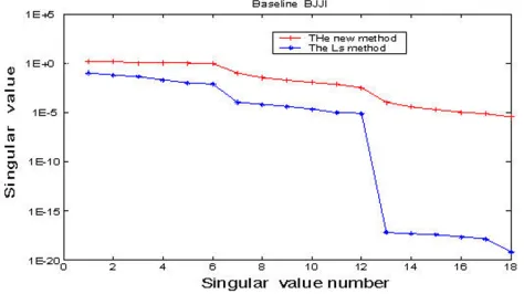
Fig. 2. A comparison of the singular values of the normal equation between the new method and the Least Squares (LS).
3.2 The construction of the regularized matrix
Since only two epochs’ observations are adopted in Eq. (4), the condition number of the normal matrixATP A
is very large (usually > 106); i.e., the normal matrix in Eq. (4) is seriously ill-conditioned (Hoerl and Kennard, 1970a, b; Ou, 2004). To solve this problem, Eq. (3) may be resolved based on the following Tikhonov regularization theorem (Tikhonov, 1977): whereαis a regularized parameter;Ris a regularized ma-trix;(X)is a stable function;|| • ||denotes the Euclidean 2-norm.
AlthoughRcan be selected as a unit matrix (Hoerl and Kennard, 1970a, b) or a positive semi-definitive matrix (Xu and Rummel, 1994; Xuet al., 2006), we would assume and directly use the prior information on the (known) reference coordinates to defineR. The matrixRis given as follows (see also Ou, 2004; Ou and Wang, 2004; Wanget al., 2006;
whereRX can be determined by the following equation
RX =diag(A
diagonal elements of the matrix. Thus, the stable function
baseline for two epochs, i.e.,XC =
XT mXTm+1
T
) can be obtained. Note that the coordinate components of the base-lines are rather accurate. If they are used as initial values of the linearization process of the observation equation,XC should be a small quantity. XT
CRXXC is also a very small
3.3 Determination of the regularized parameter
The other key problem is how to determine the regular-ized parameterα. Several methods for selectingαare intro-duced and reviewed by Xu (1992, 1998) and Hansen (2001). However, in this paper, a new scheme should be investigated to determine the regularized parameterαsince the regular-ization matrixRof this method is not positively definitive.
If different values of the regularized parameter α are given, different systematic error estimates can be obtained by the following equation:
A series of Xˆi values, corresponding to different αi
(10−15 < α
i < 102), can be obtained. Based on the
re-sults of many numerical examples associated with different baselines and satellite pairs, the estimated systematic errors are found to be less affected by the selection ofαiin a wide
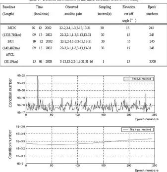
Fig. 3. Variation of the condition numbers of the LS and the new methods with time.
Fig. 4. Estimates of the systematic errors for satellite pair 22-2 of BJDX baseline (baseline length: 1338.71 km).
The relationship betweenαand the estimated systematic errors (for different satellite pairs) is shown in Fig. 1 where two baseline are used (see Section 4.2). From Fig. 1, we see that the systemic errors level out for 10−12 < α <102, suggesting thatαcan be selected as 1 in order to calculate it conveniently. Forα = 1, an example is given from the baseline BJJI (see 4.1 and Table 1).
The distribution of the singular values of the normal ma-trix of both LS and the new methods are shown in Fig. 2.
Figure 2 shows that six singular values of the LS normal equation are less than 10−15. This indicates that the LS nor-mal matrix is close to singularity. However, all singular values of the normal equation of the new method are always more than 10−5, which suggests that the singularity state of the new method is improved significantly.
In addition, the condition numbers of the normal equation of the LS and of the new method are calculated using all 245 epochs of data for BJJI baseline. Their variation with time is shown in Fig. 3. At the top of Fig. 3, all condition numbers of the LS normal equation are more than 1017, and at the bottom of this figure, all condition numbers of the new method normal equation are less than 104 and their deviations are very stable. This distribution shows that the state of the ill-conditioned equation can be well controlled using the new method and that the systematic errors may be estimated in two epochs each time by Eqs. (6) and (7). For a long-term observation, the sequential values of the estimated systematic errors can be obtained.
4.
Results and Analyses of the Experiments
4.1 Data background
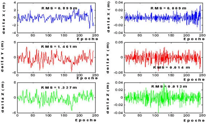
Fig. 5. A comparison of the deviations of the baseline components with and without the systematic errors uncorrected using the new method for BJDX baseline (09/12/2002).
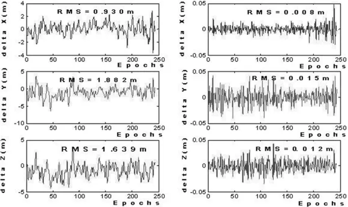
Fig. 6. A comparison of the deviations of the baseline components with and without the systematic errors corrected using the new method for BJDX baseline (09/13/2002).
Fig. 7. The estimates of the systematic errors for satellite pair 22-2 of BJJI baseline.
Tientsin) is a medium-long baseline (149.489 km). These two baselines are from Crustal Movement Observations Network of China (CMONC) observed on 12 September 2003 and 13 September 2002, respectively, with a 30-s sam-pling interval and 15◦elevation cut-off angle. The satellite pairs are PRN 22-2, 2-1, 1-3, 3-13, and 13-31, and there are 245 epochs of data in the observation. The baseline AVCL is a short baseline (38.190 km) from the AVCA sta-tion to the CLRE stasta-tion in the Nasta-tional CORS located in the Michigan area in the USA. It was observed on 15 June, 2003, with a 1-s sampling interval and 15◦elevation cut-off angle. The satellite pairs are PRN 3-13, 13-2, 2-1, 1-31, and 31-16, and there are 3500 epochs of data in the observation.
4.2 Data processing scheme
Fig. 8. A comparison of the deviations of the baseline components with and without the systematic errors corrected using the new method for BJJI baseline (09/12/2002).
Fig. 9. A comparison of the deviations of the baseline components with and without the systematic errors uncorrected using the new method for BJJI baseline (09/13/2002).
Fig. 10. Estimates of the systematic errors for satellite pair 22-2 of AVCL baseline.
epoch, etc.). The systematic errors are then calculated for each unit using Eq. (7).
4.3 Results and analysis
For the baseline BJDX, we estimated the systematic er-rors in two adjacent days using our new method. Figure 4 represents the estimates of the systematic errors of the satel-lite pair 22-2. From Fig. 4, it can be seen that the maximum systematic error estimates is as high as 3 m and the mini-mum exceeds−3 m. The root mean square (RMS) error is more than several decimeters.
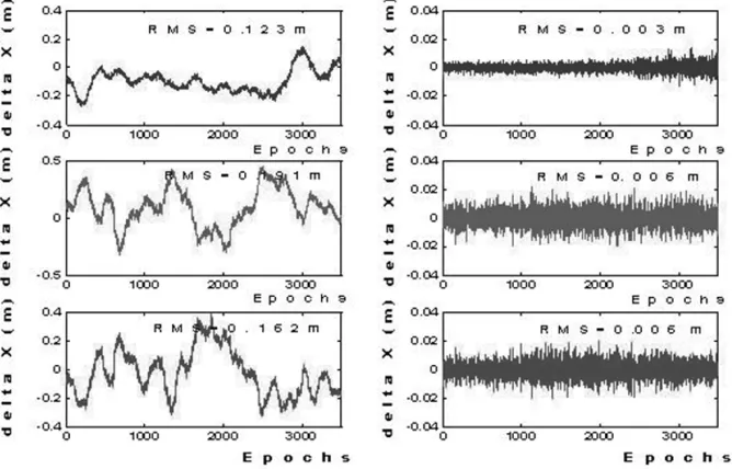
sys-Fig. 11. A comparison of the deviations of the baseline components with and without the systematic errors corrected using the new method for AVCL baseline.
tematic errors on any new station(s); this holds true for all of the following comparisons). The RMS of uncorrected systematic errors in the coordinate components of the base-lines is obviously larger than that of those basebase-lines with the systematic errors corrected. The RMS of the latter is at the level of centimeters, which reflects the precision of the coordinates of the reference stations and suggests that the systematic errors have been eliminated successfully using the new approach.
The systematic errors are also estimated for the baseline BJJI using two adjacent days of data. The estimates of the systematic errors of the satellite pair 22-2 are shown in Fig. 7.
The estimates of the systematic errors of this baseline have characters that are similar to those of the baseline BJDX. A comparison of the coordinate components of the baseline without the systematic errors corrected and with the systematic errors corrected is shown in Figs. 8 and 9, respectively.
For the baseline AVCL, whose sampling interval is 1 s, there are more epochs of data. The estimates of the system-atic errors of the satellite pair 31-16 are shown in Fig. 10. The estimates of the systematic errors of this baseline are at the level of decimeters. A comparison of the estimates of the components of the baseline with and without the sys-tematic errors corrected is shown in Fig. 11. It can be seen that the precision (RMS) of the coordinate components with the systematic errors corrected is at the level of millime-ters, while the precision (RMS) of the coordinates’ compo-nents without the systematic errors corrected at the decime-ter level.
Based on these results, it can be concluded that the sys-tematic errors are not negligible for medium-long baselines and that an effective measure must be taken to remove them. Positioning accuracy can be improved significantly after the systematic errors are identified. A centimeter-level of pre-cision can be achieved for the coordinates of the baselines
when the systematic errors are properly corrected. These results show that the estimation process of the systematic errors is very successful and that the new approach is effec-tive.
5.
Conclusions
This paper presents a new method for estimating the sys-tematic errors for medium-long baseline GPS data process-ing. The proposed method uses several epochs or as few as only two adjacent epochs of GPS data for the calculation. Two key steps are adopted. First, the systematic errors are considered to be unknown parameters to be estimated. It should be noted that the systematic errors mentioned here are the combined residual errors, which include the residu-als of the tropospheric delays and the other unmodeled er-rors. Secondly, the code and the phase difference between two adjacent epochs are regarded as basic measurements. The new method is markedly different from existing meth-ods in that it effectively combines the Tikhonov regular-ization principle with a scheme designed for constructing the regularized matrix. It also determines the correspond-ing regularized parameter based on the information of the known coordinates of the reference stations. Through the application of these steps, the new method can improve the state of the ill-posed problem of the normal equation matrix and estimate the systematic errors precisely and reliably.
Acknowledgments. The data used here were provided by the Crustal Motion Observation Network of China and the National CORS in the Michigan area network of the USA. We would like to thank the associate editor, reviewers, and Dr. Xu Peiliang for suggestions that improved this paper. We also thank the Na-tional Natural Science foundation of China 908 project and from the scientific research fund of the Second Institute of Oceanog-raphy, SOA for financial support (grant #40674012, 40474009, 40625013, 40776036 and 908 ZC-I-06).
References
USA, 519–528, 1996.
Dai, L., J. L. Wang, C. Rizos, and S. W. Han, Predicting atmospheric biases for real-time ambiguity resolution in GPS/GLONASS reference station networks,J. Geod.,76, 617–628, 2003.
Fotopoulos, G. and M. E. Cannon, Spatial and temporal characteristics of DGPS carrier phase errors over a regional network,Proc. U.S. Institute of Navigation Annual Meeting, San Diego, California, 26–28, June, 54– 64, 2000.
Gao, Y., Z. Li, and J. F. McLellan, Carrier phase based regional area differential GPS for decimeter-level positioning and navigation,Proc 10th Int Tech Meeting Satellite Division Inst Navigation, Kansas City, Mo, 16–19 September, 1305–1313, 1997.
Han, S. and C. Rizos, GPS network design and error mitigation for real-time continuous array monitoring system,Proc. of 9th Int. Tech. Meeting of the Satellite Division of the U.S. Inst. of Navigation, Kansas City, Missouri, 17–20 September, 1827–1836, 1996.
Hansen, P. C., The L-Curve and its Use in the Numerical Treatment of In-verse Problems,Computational Inverse Problems in Electrocardiology, 5, 119–142, WIT Press, 2001.
Hoerl, A. E. and R. W. Kennard, Ridge regression: Biased estimation for non-orthogonal problems,Technometrics,12, 55–67, 1970a.
Hoerl, A. E. and R. W. Kennard, Ridge regression: Applications to non-orthogonal problems,Technometrics,12, 69–82, 1970b, correction,12, 123.
Hofmann, B. W., H. Lichtenegger, and J. Collins,Global positioning sys-tem: theory and practice, 5th Edition, Springer, Berlin Heidelberg New York, 2001.
Horemuˇz, M. and L. E. Sj¨oberg, Rapid GPS ambiguity resolution for short and long baselines,J. Geod.,76, 381–391, 2002.
Hu, G. R., H. S. Khoo, P. C. Goh, and C. L. Law, Development and assessment of GPS virtual reference stations for RTK positioning,J. Geod.,77, 292–302, 2003.
Lachapelle, G., P. Alves, L. P. Fortes, M. E. Cannon, and B. Townsend, DGPS RTK positioning using a reference network,Proc of the 13th Int Tech Meeting Satellite Division US Inst Navigation, Salt Lake City, UT, 19–22 September, 1165–1171, 2000.
Landau, H., U. Vollath, and X. M. Chen, Virtual Reference Station Sys-tems,J. GPS,1.1, 137–144, 2003.
Leick, A.,GPS satellite surveying, 3rd Edition, Wiley, New York, 2004. Odijk, D., H. van der Marel, and I. Song, Precise GPS positioning by
Teunissen, P. J., The geometry-free GPS ambiguity search space with a weighted ionosphere,J. Geod.,71, 370–383, 1997.
Tikhonov, A. N. and V. Y. Arsenin,Solutions of Ill-posed Problems, New York: Wiley, 10–21, 1977.
Vollath, U., A. Buerchl, H. Landau, C. Pagels, and B. Wagner, Long-Range RTK Positioning Using Virtual Reference Stations,Proc. of the 13th Int. Tech. Meeting Satellite Division US Inst Navigation, September, Salt Lake City, USA, 1143–1147, 2000.
Vollath, U., H. Landau, X. Chen, K. Doucet, and C. Pagels, Network RTK versus Single Base RTK—Understanding the Error Characteris-tics,Proc. of the 15th Int. Tech. Meeting Satellite Division US Inst. Nav-igation, 24–27 September, Portland USA, 2774–2781, 2002.
Wang, Z., C. Rizos, and S. Lim, Single epoch algorithm based on Tikhonov regularization for deformation monitoring using single frequency GPS receivers,Surv. Rev.,38, 682–688, 2006.
Xu, P. L., The Value of Minimum Norm Estimation of Geopotential Fields,
Geophys. J. Int.,111, 170–178, 1992.
Xu, P. L., Truncated SVD Methods for Linear Discrete Ill-posed Problems,
Geophys. J. Int.,135, 505–514, 1998.
Xu, P. L. and R. Rummel, A Generalized Ridge Regression Method with Applications in Determination of Potential Fields,Manuscr. Geod.,20, 8–20, 1994.
Xu, P. L., Y. Fukuda, and Y. M. Liu, Multiple Parameter Regularization: Numerical Solutions and Applications to the Determination of Geopo-tential from Precise Satellite Orbits,J. Geod.,80, 17–27, 2006. Yang, Y., Robust estimation of geodetic datum transformation,J. Geod.,
73, 68–274, 1999.
Zhang, K., F. Wu, S. Wu, C. Rizos, C. Roberts, L. Ge, T. Yan, C. Gor-dini, A. Kealy, M. Hale, P. Ramm, H. Asmussen, D. Kinlyside, and P. Harcombe, Sparse or Dense: Challenges of Australian Network RTK,
Proceedings of IGNSS Symposium 2006, Holiday Inn Surfers Paradise, Australia, 17–21, July 2006.
Zhou, J. W., J. K. Ou, and Y. X. Yang,Research on the theory of observa-tion data and errors, 29–35, Seismic Publishing House, Beijing, 1999 (in Chinese).