R E S E A R C H
Open Access
An extrapolation full multigrid algorithm
combined with fourth-order compact
scheme for convection–diffusion equations
Ming Li
1,2, Zhoushun Zheng
1and Kejia Pan
1**Correspondence:
1School of Mathematics and
Statistics, Central South University, Changsha, P.R. China
Full list of author information is available at the end of the article
Abstract
In this paper, we propose an extrapolation full multigrid (EXFMG) algorithm to solve the large linear system arising from a fourth-order compact difference discretization of two-dimensional (2D) convection diffusion equations. A bi-quartic Lagrange interpolation for the solution on previous coarser grid is used to construct a good initial guess on the next finer grid for V- or W-cycles multigrid solver, which greatly reduces the number of relaxation sweeps. Instead of performing a fixed number of multigrid cycles as used in classical full multigrid methods, a series of grid level dependent relative residual tolerances is introduced to control the number of the multigrid cycles. Once the fourth-order accurate numerical solutions are obtained, a simple method based on the midpoint extrapolation is employed for the fourth-order difference solutions on two-level grids to construct a sixth-order accurate solution on the entire fine grid cheaply and directly. Numerical experiments are conducted to verify that the proposed method has much better efficiency compared to classical multigrid methods. The proposed EXFMG method can also be extended to solve other kinds of partial differential equations.
MSC: 65N06; 65N55
Keywords: Extrapolation; Full multigrid method; Compact difference scheme; Convection–diffusion equation
1 Introduction
Richardson extrapolation [1, 2] is an acceleration method, used to improve the rate of con-vergence for a sequence. In 1983, Marchuk and Shaidurov extended Richardson extrapo-lation technique in the framework of the finite difference (FD) method [3]. Later on, Blum et al. discussed Richardson extrapolation strategy in conjunction with the finite element (FE) method [4–7].
Multigrid methods (MGs) [8, 9] have been shown to be one of the most efficient modern numerical strategies to solve the large linear systems arising from FE or FD discretizations of partial differential equations (PDEs), such as the Poisson equation [10–14], Helmholtz equation [15–17], convection–diffusion equation [18–20]. The main advantage of the multigrid method is that its convergence rate is independent of the number of unknowns [8, 21]. The full multigrid (FMG) method, which combines nested iteration with a V- or W-cycles multigrid method, is well known to be optimal with respect to the energy norm
and theL2-norm [8, 21–23]. It starts on the coarsest grid with a direct solver, then the solution is interpolated to form the initial guess on the next finer grid, where a few V-or W-cycles are used to produce an approximate solution whose algebraic errV-or matches with the discretization error. The procedure goes on recursively until the finest grid.
Recently, the Richardson extrapolation technique has been applied in multigrid meth-ods. One group of researchers used Richardson extrapolation to construct a good initial guess for the iterative solver. An extrapolation cascadic multigrid (EXCMG) method [24, 25] was proposed by Chen et al. to solve second-order elliptic problems. This method uses a new extrapolation formula to construct a quite good initial guess for the iterative solu-tion on the next finer grid, which greatly improves the convergence rate of the original CMG algorithm (see [24–26] for details). Then the EXCMG method has been success-fully applied to non-smooth elliptic problems [27, 28], parabolic problems [29], and some other related problems [30–32]. Moreover, Pan [33] and Li [34, 35] developed some EX-CMG methods combined with high-order compact difference schemes to solve Poisson equations. In 2017, Hu et al. [36] obtained the super-optimality of the EXCMG method under the energy norm forH2+α-regular (0 <α≤1) elliptic problems.
Another group of researchers made efforts to design an iterative procedure with Richardson extrapolation strategy to enhance the solution accuracy on the finest grid. Sun, Zhang and Dai developed a sixth-order FD scheme for solving the 2D convection– diffusion equation [37, 38]. In their approach, the ADI method is applied to compute the fourth-order accurate solution on the fine and coarse grids, respectively, then the Richard-son extrapolation technique and an operator-based interpolation scheme are employed in each ADI iteration to calculate the sixth-order accurate solution on the fine grid. In 2009, Wang and Zhang designed an explicit sixth-order compact discretization strategy (MG-Six) for the 2D Poisson equation [39]. They used a V-cycle multigrid method to get the fourth-order accurate solutions on both the fine and the coarse grids first, and then chose the iterative operator with Richardson extrapolation technique to compute the sixth-order accurate solution on the fine grid.
We extend the idea described in the literature [32, 33, 39] to the original full multigrid method, and develop an extrapolation full multigrid (EXFMG) method to solve the 2D convection–diffusion equation with a fourth-order compact difference discretization. To be more precise, a bi-quartic Lagrange interpolation operator on a coarser grid is applied to get a good initial guess on the next finer grid for the multigrid V- or W-cycles solver. Besides, a stopping criterion related to relative residual is used to conveniently obtain the numerical solution with the desired accuracy. Moreover, a mid-point extrapolation strat-egy is used to obtain cheaply and directly a sixth-order accurate solution on the entire fine grid from two fourth-order solutions on two different grids (current fine and previous coarse grids). Finally, through two examples chosen from the literature, the computational efficiency of the EXFMG method is discussed in detail.
2 Model problem and discretization
Consider the following two-dimensional (2D) convection–diffusion equation:
–uxx(x,y) –uyy(x,y) +p(x,y)ux(x,y) +q(x,y)uy(x,y) =f(x,y), (x,y)∈, (1)
with suitable Dirichlet boundary conditions. Hereis a rectangular domain,p(x,y) and
q(x,y) are the given convection velocities,f(x,y) is the given source term, andu(x,y) is the unknown function. All these functions are assumed to be sufficiently smooth and have the necessary continuous partial derivatives up to certain orders. This equation is used to describe many processes in fields of fluid dynamics.
Let= [0,Mx]×[0,My] and divideintoNx×Nyuniform grids with the mesh size x=MxNx andy=MyNy in thexandycoordinate directions, respectively.NxandNyare
the numbers of uniform intervals in thexandydirections, respectively. The mesh points are (xi,yj) withxi=ixandyi=iy, 0≤i≤Nx, 0≤j≤Ny. For simplicity, we useUi,j
to represent the approximation ofu(xi,yj) at the mesh point (xi,yj), setfi,j=f(xi,yj),pi,j=
p(xi,yj), and so on.
Hi,j=qi,j+ x2
12
(qxx)i,j– (pqx)i,j
+y 2
12
(qyy)i,j– (qqy)i,j
,
Fi,j=fi,j+ x2
12
(fxx)i,j– (pfx)i,j
+y 2
12
(fyy)i,j– (qfy)i,j
. (3)
Now seth1=x=yand assume that the domain is divided into a sequence of gridsk,k= 1, 2, . . . ,Lwith mesh sizehk=h1/2k–1. By applying the fourth-order compact
scheme (2), we obtain the corresponding sparse linear system,
Akuk=Fk, k= 1, 2, . . . ,L, (4)
whereAkis a nine-diagonal matrix,Fkandukare the right-hand side vector and the
solu-tion vector, respectively.
3 Classical multigrid method
The multigrid (MG) method is a very efficient approach to solving large sparse linear sys-tems arising from FE or FD discretizations of various PDEs [8]. The main feature behind the MG method is to divide the errors into high frequency components and low frequency components and eliminate them in different grids. To be more specific, the high frequency component errors are eliminated on the fine grid, while the remaining low frequency er-rors are eliminated by a recursive procedure on the coarse grid. We depict this method in Algorithm 1, in which a direct solver “DSOLVER” is used on the coarsest grid, since the size of the linear system is small. A restriction operatorRjj+1(such as a full-weighting scheme) is employed to project residual from the fine grid to the coarse grid, and an inter-polation operatorIjj+1(such as bilinear interpolator) is used to transfer corrections from the coarse grid to the fine grid. The recursion parameterNcyclesis greater than or equal to one. If Ncycles = 1, the so-called V-cycle is generated, while Ncycles = 2 leads to the W-cycle. A cycle of Algorithm 1, means that it starts from the finest grid to the coarsest grid and back to the finest grid again. When Algorithm 1 is applied to the finest grid sys-tem (2) in the solution of which we are interested, it can be repeated until the accuracy of approximation on the finest grid is considered to be high enough.
Algorithm 1Classical multigrid method:uL⇐MGM(AL,u0L,FL,L)
1: Setj←L– 1
2: Pre-smoothingv1times:uvj+11 ⇐Smoothv1(Aj+1,u0j+1,Fj+1)
3: Restricting:rj⇐Rjj+1(Fj+1–Aj+1uvj+11 )
4: ifj== 1 (Coarsest grid) , then
5: e1⇐DSOLVER(A1e1=r1)
6: else
7: Sete0j ←0 8: fori= 1,Ncyclesdo
9: ej⇐MGM(Aj,e0j,rj,j),
10: Correcting:u¯j+1←uvj+11 +I
j+1
j ej
Algorithm 2Full multigrid method (FMG)
1: u∗1⇐DSOLVER(A1u1=F1)
2: forj= 2, 3, . . . ,Ldo
3: Compute an initial guess:u0j ⇐Pjj–1u∗j–1 Pjj–1is a FMG interpolation operator 4: Solveu∗j by performingkjtimesj-grid cycles using the initial approximationu0j
u∗j ⇐MGMkjAj,u0j,Fj,j
In fact, Algorithm 1 can be incorporated with the classical FMG method naturally. The FMG method starts with the coarsest grid, and uses an interpolation operatorPjj–1to pro-duce an initial guess for Algorithm 1 on the next finer grid; see Algorithm 2 for details. The interpolation operatorPjj–1 usually is of higher accuracy than the interpolation operator
Ijj–1used within the multigrid iteration. It is well known that FMG delivers an approxima-tion up to discretizaapproxima-tion accuracy if the multigrid cycle converges satisfactorily and if the order of FMG interpolation is larger than the discretization order of the PDE [8].
4 Extrapolation full multigrid method 4.1 Description of the EXFMG algorithm
In this section, we shall establish an extrapolation full multigrid (EXFMG) method to solve the 2D convection–diffusion equation (1) with the fourth-order compact discretization (2). Similar to FMG method, the EXFMG method starts with the coarsest grid to compute the solution by a direct solver, and applies an interpolation operator on the current grid to provide an initial guess for Algorithm 1 on the next finer grid. Besides, EXFMG method employs a fine mesh Richardson extrapolation technique [33] to get an extrapolation so-lution on each grid, when the two soso-lutions with fourth-order accuracy on current and previous grids has been obtained by the Algorithm 1. The detailed algorithm is stated in Algorithm 3, whereFMREdenotes a fine mesh Richardson extrapolation operator which will be defined and discussed in Sect. 4.2,u¯∗i andu∗j denote the numerical solution and extrapolated solution on the gridi, respectively.
The key ingredients of this new method which are the main differences between the existing FMG methods include:
(1) A bi-quartic Lagrange interpolation operator on coarse grid is taken as a full interpolation to provide a good initial guess on the next finer grid for multigrid iteration.
(2) Instead of performing a fixed number of multigrid iterations at each level of grid as used in the usual FMG method, a tolerancejrelated to the relative residual is used
onjth grid level (see line 4 in Algorithm 3), which enables us to conveniently calculate the approximate solution with the desired accuracy and keep suitable computational cost.
Algorithm 3Extrapolation full multigrid method (EXFMG)
1: Calculate the solutionu¯∗1by a direct solver
2: forj= 2, 3, . . . ,Ldo
3: Compute an initial guess:u0j ⇐Pjj–1u¯∗j–1 Pjj–1is Bi-quartic Lagrange
interpolation operator [33]
4: Solveu¯∗j by performingj-grid cycles until jdenotes a given tolerance Fj–Aju¯j∗≤jFj
5: Richardson Extrapolation: FMREdenotes fine mesh Richardson extrapolation operator
u∗j ⇐FMREu¯∗j–1,u¯∗j
6: Output allu¯∗j andu∗j
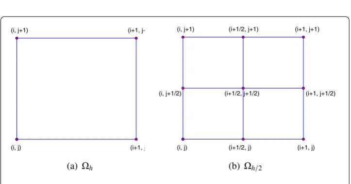
Figure 1Cells of coarse gridh(a)and refined gridh/2(b)
4.2 Fine mesh extrapolation operator
In the classical Richardson extrapolation formula, two solutions on fine and coarse grids are used to obtain an extrapolation solution on the coarse grid. Based on the Richard-son extrapolation technique and interpolation theory, in 2017, Pan proposed a mid-point extrapolation technique to enhance the accuracy of approximations on fine grid directly and cheaply (see [33] for details). Now, we will introduce this strategy for 2D case in the following.
Assume that the notationsuhanduh/2represent the fourth-order accurate solutions on coarse gridhand fine gridh/2with mesh sizehandh/2, respectively. For simplicity of description, we take a coarse cellIi,j= [xi,xi+1]×[yj,yj+1] of gridh (see Fig. 1), useuhi,j
anduhi,/2j to represent the fourth-order accurate solutions on the point (xi,yj) of the coarse
To obtain an extrapolation solution on the fine grid h/2, we first use the classical
Richardson extrapolation formula,
Eus,t=
16 15u
h/2
s,t –
1 15u
h
s,t, s=i,i+ 1,t=j,j+ 1, (5)
to get an extrapolation solution on the nodes (xs,yt). Then we apply the mid-point
extrap-olation formula [33] for those nodes (xs,yj+1/2), (xi+1/2,yt) and (xi+1/2,yj+1/2), to obtain some
formulas as follows:
Eus,j+1/2=uhs,/2j+1/2+ 1 30
uh/2–uhs,j+uh/2–uhs,j+1, s=i,i+ 1, (6)
Eui+1/2,t=uhi+1/2,/2 t+
1 30
uh/2–uhi,t+uh/2–uhi+1,t, t=j,j+ 1, (7)
Eui+1/2,j+1/2=uhi+1/2,/2 j+1/2+ 1 60
uh/2–uhi,j+uh/2–uhi+1,j+uh/2–uhi,j+1
+uh/2–uhi+1,j+1, (8)
in order to construct the corresponding extrapolation solution, respectively.
Taking the above four extrapolation formulas (5), (6), (7) and (8), we can obtain an ex-trapolation solutionEu, which is more accurate than the fourth-order accurate numerical solutionuh/2on the fine grid
h/2. For simplicity, we denote this procedure fromuh,uh/2 toEuas an operator, we call it as fine mesh Richardson extrapolation (FMRE) interpolator
Eu⇐FMRE(uh,uh/2). (9)
Remark4.1 It should be noted that the extrapolation interpolatorFMREis a local opera-tion, which can be done very effectively.
4.3 Computational work
Throughout this paper, when using Algorithm 1 as a solver on each grid of the EXFMG method, we always setNcycles= 1. Now we turn to estimate the computational cost of the EXFMG method in terms ofwork units(WUs). Roughly speaking, “1 WU” is the com-putational cost of performing one relaxation sweep on the finest grid. For simplicity, we neglect the amount of work needed to solve the equations on the coarsest grid and the transfer operators (include interpolation and restriction) between different levels of grids since it normally counts 10–20%of the total cost of the algorithm.
Assume that themjis the number of the MG cycles required on the gridjwhen the
MG solution satisfies the stopping criterion (see line 4 in Algorithm 3). Based on the above conditions, we can estimate the computational work of EXFMG withLlevels of grids for
d-dimensional problems as follows:
WUEXFMG≈(v1+v2)
mL+ (mL+mL–1)2–d+· · ·+ (mL+mL–1+· · ·+m2)2–(L–2)d
= (v1+v2)
L
j=2
L
i=j
5 Numerical experiments
In this section, we conduct numerical experiments with two examples both on the unit square domain= (0, 1)×(0, 1). In the two test problems, the right-hand side function
f(x,y) and the Dirichlet boundary conditions on∂are prescribed to satisfy the given analytic solutionsu(x,y). Our codes are written in Matlab and the programs are carried out on a desktop with Inter (R) Core(TM) i5-6200 U CPU (2.30 GHZ, 2.40 GHZ) and 4 GB RAM.
For comparison purposes, we denote the Algorithm 1 with Ncycles= 1 asMG. The it-erative procedure of MGmethod starts with zero initial guesses and terminates when the approximation solution u∗L on the finest grid satisfies the same stopping criterion FL–ALuL∗ ≤LFLas the EXFMG algorithm.
In MG and EXFMG methods withLembedded grids, the standard bilinear interpolation is used to transfer corrections from the coarse grid to the fine grid, the full-weighting scheme is employed to project residual from the fine grid to the coarse grid, the Conjugate Gradient (CG) method is chosen as a smoother to eliminate the high frequency error, and the number of pre-smoothing and post-smoothing steps are set to bev1=v2= 2.L= 10–10
is taken as the stopping tolerance on the finest grid.
In all numerical experiments, we use the notations u,u¯∗j andu∗j to denote the exact solution, numerical solution and extrapolation solution on the gridj, respectively. For
convenience of comparison, we choose theL∞-norm and theL2-norm to measure the error betweenu∗j (oru¯∗j) andu, which are defined as
u–u∗j∞=ej∞= max
(x,y)∈j
ej(x,y),
u–u∗j2=ej2=hj
(x,y)∈j
ej(x,y)2.
We also apply the definition
Order =log(ej–1/ej) log(hj–1/hj)
, j= 2,· · ·,L,
to represent the convergence order of the approximate solution. Here, · is a given norm (such asL∞,L2). Besides, we use “CPU” , “WU” and “Tflops” to record the algorithm’s computational time in seconds, work units [8] and number of flops measured inTeraFlops, respectively. “Iter” denotes the number of multigrid cycles required.
Example5.1 ([41, 42]) Consider the following differential equation:
–uxx(x,y) –uyy(x,y) +
1
ε(1 +y)uy(x,y) =f(x,y), (11) with suitable Dirichlet boundary condition and right-hand side termf(x,y), such that the exact solution is
Table 1 Errors and costs of algorithms withL= 5 for different discretization system arising from Example 5.1
L Method u–u∗L∞ u–u∗L2 CPU Iter WU Tflops
256×256 MG 6.30E–06 2.41E–06 0.92 9 47.8 1.5
EXFMG 1.23E–07 2.17E–08 0.91 6, 8, 10, 1 45.6 1.1
512×512 MG 3.94E–07 1.51E–07 3.42 9 47.8 23.5
EXFMG 2.05E–09 3.41E–10 3.05 6, 7, 9, 1 43.9 16.8
1024×1024 MG 2.47E–08 9.45E–09 14.3 9 47.8 377.9
EXFMG 7.10E–11 6.33E–12 12.1 5, 7, 8, 1 38.3 229.3
2048×2048 MG 1.54E–09 5.91E–10 43.4 10 53.1 6736.5
EXFMG 7.34E–12 8.68E–13 40.5 5, 7, 8, 1 38.3 3679.8
Table 2 Errors and costs of algorithms withL= 5 for different discretization system arising from Example 5.2
L Method u–u∗L∞ u–u∗L2 CPU Iter WU Tflops
256×256 MG 3.15E–05 3.46E–06 0.92 8 42.5 1.3
EXFMG 3.02E–06 2.84E–07 1.21 7, 9, 11, 1 52.5 1.2
512×512 MG 1.94E–06 2.13E–07 4.34 9 47.8 23.5
EXFMG 6.18E–08 4.40E–09 3.95 5, 8, 10, 1 40.3 14.4
1024×1024 MG 1.21E–07 1.33E–08 14.95 8 42.5 335.9
EXFMG 1.78E–09 3.38E–10 12.47 4, 6, 9 , 1 32.0 184.8
2048×2048 MG 7.53E–09 8.35E–10 40.64 8 42.5 5389.2
EXFMG 3.65E–10 8.29E–11 41.84 4, 5, 7, 1 30.1 2920.2
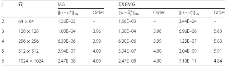
Table 3 Comparison of theL∞errors and convergence order on different grid level of MG and EXFMG methods for Example 5.1
j j MG EXFMG
u–u∗j∞ Order u–u¯∗j∞ Order u–u∗j∞ Order
2 64×64 1.56E–03 – 1.56E–03 – 3.44E–04 –
3 128×128 1.00E–04 3.96 1.00E–04 3.96 6.96E–06 5.63
4 256×256 6.30E–06 3.99 6.30E–06 3.99 1.23E–07 5.83
5 512×512 3.94E–07 4.00 3.94E–07 4.00 2.04E–09 5.91
6 1024×1024 2.47E–08 4.00 2.47E–08 4.00 7.10E–11 4.84
Example5.2 ([40]) Consider the convection–diffusion equation:
–uxx(x,y) –uyy(x,y) +x(x– 1)(1 – 2y)ux(x,y) +y(y– 1)(1 – 2x)uy(x,y) =f(x,y), (13)
with the analytic solution
u(x,y) =exp–2000(x– 0.5)2–y2. (14) The numerical results for Example 5.1 and 5.2 obtained by MG and EXFMG methods with five embedded grids are listed in Tables 1 and 2. When fixing 32×32 as the coarsest grid1, Tables 3–8 list the numerical results of EXFMG method with the stopping criteria
Table 4 Comparison of theL∞errors and convergence order on different grid level of MG and EXFMG methods for Example 5.2
j j MG EXFMG
u–u∗j∞ Order u–u¯∗j∞ Order u–u∗j∞ Order
2 64×64 1.16E–02 – 1.16E–02 – 4.14E–01 –
3 128×128 5.36E–04 4.43 5.36E–04 4.43 2.01E–04 11.01
4 256×256 3.15E–05 4.09 3.15E–05 4.09 3.02E–06 6.06
5 512×512 1.94E–06 4.02 1.94E–06 4.02 6.18E–08 5.61
6 1024×1024 1.21E–07 4.01 1.21E–07 4.01 1.78E–09 5.12
Table 5 Comparison of theL2errors and convergence order on different grid level of MG and EXFMG methods for Example 5.1
j j MG EXFMG
u–u∗j∞ Order u–u¯∗j∞ Order u–u∗j∞ Order
2 64×64 5.97E–04 – 5.97E–04 – 7.81E–05 –
3 128×128 3.84E–05 3.96 3.84E–05 3.96 1.35E–06 5.85
4 256×256 2.41E–06 3.99 2.41E–06 3.99 2.17E–08 5.96
5 512×512 1.51E–07 4.00 1.51E–07 4.00 3.41E–10 5.99
6 1024×1024 9.45E–09 4.00 9.45E–09 4.00 6.27E–12 5.77
Table 6 Comparison of theL2errors and convergence order on different grid level of MG and EXFMG methods for Example 5.2
j j MG EXFMG
u–u∗j∞ Order u–u¯∗j∞ Order u–u∗j∞ Order
2 64×64 1.37E–03 – 1.37E–03 – 1.59E–01 –
3 128×128 5.85E–05 4.55 5.85E–05 4.55 2.23E–05 12.80
4 256×256 3.46E–06 4.08 3.46E–06 4.08 2.84E–07 6.29
5 512×512 2.13E–07 4.02 2.13E–07 4.02 4.40E–09 6.01
6 1024×1024 1.33E–08 4.00 1.33E–08 4.00 3.38E–10 3.70
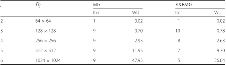
Table 7 Comparison of the iteration number and computational cost (WU) on different grid level of MG and EXFMG methods for Example 5.1
j j MG EXFMG
Iter WU Iter WU
2 64×64 1 0.02 1 0.02
3 128×128 9 0.70 10 0.78
4 256×256 9 2.95 8 2.63
5 512×512 9 11.95 7 9.30
6 1024×1024 9 47.95 5 26.64
on each gridj,j= 2, 3, . . . ,L. We also present the numerical errors and computational
Figure 2Comparison of theL∞-norm erroru–u∗L∞with different mesh sizehL(L= 6)
Figure 3Comparison of theL2-norm erroru–u∗
L2with different mesh sizehL(L= 6)
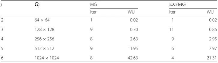
Table 8 Comparison of the iteration number and computational cost (WU) on different grid level of MG and EXFMG methods for Example 5.2
j j MG EXFMG
Iter WU Iter WU
2 64×64 1 0.02 1 0.02
3 128×128 9 0.70 11 0.86
4 256×256 8 2.63 9 2.95
5 512×512 9 11.95 6 7.97
6 1024×1024 8 42.63 4 21.31
For the accuracy, we find that the numerical solutions from the EXFMG method are much more accurate than those from the MG method (see Tables 1 and 2, Figs. 2 and 3). This means that, to achieve the same accuracy, fewer grid points are needed for the EXFMG method than for the MG method. For instance, the numerical solution by the EXFMG method on the 256×256 grid is comparable to the numerical solution obtained by the MG method on the 512×512 grid in Tables 1 and 2.
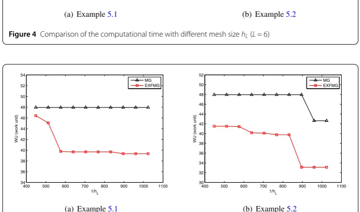
-Figure 4Comparison of the computational time with different mesh sizehL(L= 6)
Figure 5Comparison of the WU of MG and EXFMG methods withL= 6
norm while the extrapolated solutionu∗j achieves sixth-order accuracy on most levels of grids and starts to lose convergent order on fine grids since the requirement to achieve sixth-order accuracy on fine grids is much higher.
Tables 7 and 8 list computational costs on each level of grids for the EXFMG method and MG methods, we find that WU as well as the total work cost of EXFMG method depends greatly on the number of multigrid iterations on the finest gridL. From Tables 1 and 2,
we noticed that the EXFMG method takes fewer iterations on the finest grid, which is more efficient than the MG method. Therefore, the total computational cost (WU, Tflop and CPU time) of EXFMG method are much lower than that of the MG method, which is particularly true when mesh size is less or equal to 5121 (see Tables 1, 2 , 7, 8 and Figs. 4, 5 for details).
From the above discussion, we can see that the EXFMG method not only achieves high-order accuracy but also keeps a low computational cost. Hence, it is a cost-effective nu-merical solver.
6 Conclusion
convection–diffusion equation. Numerical experiments were conducted for two test prob-lems to demonstrate that the proposed EXFMG method improves the solution accuracy and keeps less computational costs, compared to the classical MG method.
We need point out that the fourth-order compact difference method, which is employed to discretize the differential equation, can be replaced by other numerical methods, such as the FE method and the finite volume method. Furthermore, we also plan to extend this study and apply EXFMG algorithm with sixth-order combined compact difference scheme [43–45] to solve unsteady three-dimensional convection–diffusion equations.
Acknowledgements
The research was supported by the National Natural Science Foundation of China (Nos. 41474103, 11661027, 11601012), the National Key Research and Development Program of China (Nos. 2017YFB0701700, 2017YFB0305601), the Excellent Youth Foundation of Hunan Province of China (No. 2018JJ1042), the Natural Science Foundation of Yunnan Province of China (No. 2017FH001-012), the Innovation-Driven Project of Central South University (No. 2018CX042) and the Reserve Talents Foundation of Honghe University (No. 2015HB0304). We are grateful to the two anonymous reviewers for their helpful comments.
Competing interests
The authors declare that they have no competing interests.
Authors’ contributions
The authors declare that the work was realized in collaboration with the same responsibility. All authors read and approved the final manuscript.
Author details
1School of Mathematics and Statistics, Central South University, Changsha, P.R. China.2Department of Mathematics,
Honghe University, Mengzi, P.R. China.
Publisher’s Note
Springer Nature remains neutral with regard to jurisdictional claims in published maps and institutional affiliations.
Received: 11 January 2018 Accepted: 3 May 2018 References
1. Richardson, L.F.: The approximate solution of physical problems involving differential equations using finite differences, with an application to the stress in a masonry dam. Philos. Trans. R. Soc. Lond. Ser. A210, 307–357 (1910) 2. Richardson, L.F.: The deferred approach to the limit. I: the single lattice. Philos. Trans. R. Soc. Lond. Ser. A226, 299–349
(1927)
3. Marchuk, G.I., Shaidurov, V.V.: Difference Methods and Their Extrapolations. Springer, New York (1983)
4. Blum, H., Lin, Q., Rannacher, R.: Asymptotic error expansion and Richardson extrapolation for linear finite elements. Numer. Math.49(1), 11–37 (1986)
5. Chen, C.M., Lin, Q.: Extrapolation of finite element approximation in a rectangular domain. J. Comput. Math.7(3), 227–233 (1989)
6. Fairweather, G., Lin, Q., Lin, Y.P., et al.: Asymptotic expansions and Richardson extrapolation of approximate solutions for second order elliptic problems on rectangular domains by mixed finite element methods. SIAM J. Numer. Anal.
44(3), 1122–1149 (2006)
7. Lin, Q., Lu, T., Shen, S.M.: Maximum norm estimate, extrapolation and optimal point of stresses for finite element methods on strogle regular triangulation. J. Comput. Math.1(4), 376–383 (1983)
8. Trottenberg, U., Oosterlee, C.W., Schller, A.: Multigrid. Academic Press, London (2001) 9. Hackbusch, W.: Multi-Grid Methods and Applications. Springer, Berlin (1985)
10. Othman, M., Abdullah, A.R.: An efficient multigrid Poisson solver. Int. J. Comput. Math.71(4), 541–553 (1999) 11. Ge, Y.B.: Multigrid method and fourth-order compact difference discretization scheme with unequal meshsizes for
3D poissson equation. J. Comput. Phys.229(18), 6381–6391 (2010)
12. Gupta, M.M., Kouatchou, J., Zhang, J.: Comparison of second and fourth order discretization for multigrid Poisson solver. J. Comput. Phys.132, 663–674 (1997)
13. Shi, Z.C., Xu, X.J., Huang, Y.Q.: Economical cascadic multigrid methods (ECMG). Sci. China Ser. A, Math.50, 1765–1780 (2007)
14. Li, C.L.: A new parallel cascadic multigrid method. Appl. Math. Comput.219, 10150–10157 (2013) 15. Elman, H.C., Ernst, O.G., O’leary, D.P.: A multigrid method enhanced by Krylov subspace iteration for discrete
Helmholtz equations. SIAM J. Sci. Comput.23(4), 1291–1315 (2001)
16. Erlangga, Y.A., Oosterlee, C.W., Vuik, C.: A novel multigrid based precondtioner for heterogeneous Helmholtz problems. SIAM J. Sci. Comput.27(4), 1471–1492 (2006)
17. Stolk, C.C., Ahmed, M., Bhowmik, S.K.: A multigrid method for the Helmholtz equation with optimized coarse grid corrections. SIAM J. Sci. Comput.36(6), A2819–A2841 (2013)
19. Gupta, M.M., Zhang, J.: High accuracy multigrid solution of the 3D convection-diffusion euqaiton. Appl. Math. Comput.113(2), 249–274 (2000)
20. Bhowmik, S.K., Stolk, C.C.: Preconditioners based on windowed Fourier frames applied to elliptic partial differential equations. J. Pseudo-Differ. Oper. Appl.2(3), 317–342 (2011)
21. Brandt, A.: Multi-level adaptive solutions to boundary-value problems. Math. Comput.31(138), 333–390 (1977) 22. Mandel, J., Parter, S.V.: On the multigrid F-cycle. Appl. Math. Comput.37(1), 19–36 (1990)
23. Thekale, A., Gradl, T., et al.: Optimizing the number of multigrid cycle in the full multigrid algorithm. Numer. Linear Algebra Appl.17(2–3), 199–210 (2010)
24. Chen, C.M., Hu, H.L., et al.: Analysis of extrapolation cascadic multigrid method (EXCMG). Sci. China Ser. A51, 1349–1360 (2008)
25. Chen, C.M., Shi, Z.C., Hu, H.L.: On extrapolation cascadic multigrid method. J. Comput. Math.29(6), 684–697 (2011) 26. Chen, C.M., Hu, H.L.: Extrapolation cascadic multigrid method on piecewise uniform grid. Sci. China Math.56(12),
2711–2722 (2013)
27. Hu, H.L., Chen, C.M., Pan, K.J.: Asymptotic expansions of finite element solutions to Robin problems inH3and their
application in extrapolation cascadic multigrid method. Sci. China Math.57, 687–698 (2014)
28. Pan, K.J., He, D.D., Chen, C.M.: An extrapolation cascadic multigrid method for elliptic problems on reentrant domains. Adv. Appl. Math. Mech.9(6), 1347–1363 (2017)
29. Hu, H.L., Chen, C.M., Pan, K.J.: Time-extrapolation algorithm (TEA) for linear parabolic problems. J. Comput. Math.32, 183–194 (2014)
30. Pan, K.J., Tang, J.T., et al.: Extrapolation cascadic multigrid method for 2.5D direct current resistivity modeling. Chin. J. Geophys.55, 2769–2778 (2012) (in Chinese)
31. Pan, K.J., Tang, J.T.: 2.5-D and 3-D DC resistivity modelling using an extrapolation cascadic multigrid method. Geophys. J. Int.197(3), 1459–1470 (2014)
32. Pan, K.J., He, D.D., et al.: A new extrapolation cascadic multigrid method for three dimensional elliptic boundary value problems. J. Comput. Phys.344, 499–515 (2017)
33. Pan, K.J., He, D.D., Hu, H.L.: An extrapolation cascadic multigrid method combined with a fourth-order compact scheme for 3D Poisson equation. J. Sci. Comput.70, 1180–1203 (2017)
34. Li, M., Li, C.L., et al.: Cascadic multigrid methods combined with sixth order compact scheme for Poisson equation. Numer. Algorithms71(4), 715–727 (2016)
35. Li, M., Li, C.L.: New cascadic multigrid methods for two-dimensional Poisson problem based on the fourth-order compact difference scheme. Math. Methods Appl. Sci.41(3), 920–928 (2018)
36. Hu, H.L., Ren, Z.Y., et al.: On the convergence of an extrapolation cascadic multigrid method for elliptic problems. Comput. Math. Appl.74, 759–771 (2017)
37. Sun, H., Zhang, J.: A high order finite difference discretization strategy based on extrapolation for convection-diffusion equations. Numer. Methods Partial Differ. Equ.20(1), 18–32 (2004)
38. Dai, R.X., Zhang, J., Wang, Y.: Higher order ADI method with completed Richardson extrapolation for solving unsteady convection-diffusion equations. Comput. Math. Appl.71, 431–442 (2016)
39. Wang, Y., Zhang, J.: Sixth order compact scheme combined with multigrid method and extrapolation technique for 2D Poisson equation. J. Comput. Phys.228, 137–146 (2009)
40. Zhang, J., Sun, H.W., Zhao, J.J.: High order compact scheme with multigrid local mesh refinement procedure for convection diffusion problems. Comput. Methods Appl. Mech. Eng.191, 4661–4674 (2002)
41. Ge, Y.B., Cao, F.J.: Multigrid method based on the transformation-free HOC scheme on nonuniform grids for 2D convection diffusion problems. J. Comput. Phys.230, 4051–4070 (2011)
42. Tian, Z.F., Dai, S.Q.: High-order compact exponential finite difference methods for convection-diffusion type problems. J. Comput. Phys.220, 952–974 (2007)
43. He, D.D., Pan, K.J.: An unconditionally stable linearized CCD-ADI method for generalized nonlinear Schrödinger equations with variable coefficients in two and three dimensions. Comput. Math. Appl.73, 2360–2374 (2017) 44. Lee, S.T., Liu, J., Sun, H.W.: Combined compact difference scheme for linear second-order partial differential equations
with mixed derivative. J. Comput. Appl. Math.264, 23–37 (2014)