R E S E A R C H
Open Access
Sensing time and power allocation for cognitive
radios using distributed Q-learning
Olivier van den Biggelaar
*, Jean-Michel Dricot, Philippe De Doncker and François Horlin
Abstract
In cognitive radios systems, the sparse assigned frequency bands are opened to secondary users, provided that the aggregated interferences induced by the secondary transmitters on the primary receivers are negligible. Cognitive radios are established in two steps: the radios firstly sense the available frequency bands and secondly
communicate using these bands. In this article, we propose two decentralized resource allocation Q-learning algorithms: the first one is used to share the sensing time among the cognitive radios in a way that maximize the throughputs of the radios. The second one is used to allocate the cognitive radio powers in a way that maximizes the signal on interference-plus-noise ratio (SINR) at the secondary receivers while meeting the primary protection constraint. Numerical results show the convergence of the proposed algorithms and allow the discussion of the exploration strategy, the choice of the cost function and the frequency of execution of each algorithm.
1. Introduction
The scarcity of available radio spectrum frequencies, densely allocated by the regulators, represents a major bottleneck in the deployment of new wireless services. Cognitive radios have been proposed as a new technol-ogy to overcome this issue [1]. For cognitive radio use, the assigned frequency bands are opened to secondary users, provided that interference induced on the primary licensees is negligible. Cognitive radios are established in two steps: the radios firstly sense the available frequency bands and secondly communicate using these bands.
To tackle the fading phenomenon–an attenuation of the received power due to destructive interferences between the multiple interactions of the emitted wave with the environment–when sensing the frequency spec-trum, cooperative spectrum sensing has been proposed to take advantage of the spatial diversity in wireless channels [2,3]. In cooperative spectrum sensing, the sec-ondary cognitive nodes send the results of their indivi-dual observations of the primary signal to a base station through specific control channels. The base station then combines the received information in order to make a decision about the primary network presence. Each cog-nitive node observes the primary signal during a certain sensing time, which should be chosen high enough to
ensure the correct detection of the primary emitter but low enough so that the node has still enough time to communicate. In literature [4,5], the sensing times used by the cognitive nodes are generally assumed to be iden-tical and allocated by a central authority. In [6], the sen-sing performance of a network of independent cognitive nodes that individually select their sensing times is ana-lyzed using evolutionary game theory.
It is generally considered in literature that the second-ary users can only transmit if the primsecond-ary network is inactive or if the secondary users are located outside a keep-out region surrounding the primary transmitter, or equivalently, if the secondary users generate an interfer-ence inferior to a given threshold on a so called protec-tion contoursurrounding the primary transmitter [7,8]. However, multiple simultaneously transmitting second-ary users may individually meet the protection contour constraint while collectively generating an aggregated interference that exceeds the acceptable threshold. In [7], the effect of aggregated interference caused by IEEE 802.22 secondary users on primary DTV receivers is analyzed. In [9], the aggregated interference generated by a large-scale secondary network is modeled and the impact of the secondary network density on the sensing requirements is investigated. In [10], a decentralized power allocation Q-learning algorithm is proposed to protect the primary network from harmful aggregated interference. The proposed algorithm removes the need * Correspondence: [email protected]
Université Libre de Bruxelles (ULB), Avenue F. D. Roosevelt 50, B-1050 Brussels, Belgium
for a central authority to allocate the powers in the sec-ondary network and therefore minimizes the communi-cation overhead. The cost functions used by the algorithm are chosen so that the aggregated interference constraint is exactly met on the protection contour. Unfortunately, the cost functions do not take into account the preferences of the secondary network.
This article aims to illustrate the potential of Q-learn-ing for cognitive radio systems. For this purpose two decentralized Q-learning algorithm are presented to solve the allocation problems that appear during the sensing phase on the one hand and during the commu-nication phase on the other hand. The first algorithm allows to share the sensing times among the cognitive radios in a way that maximize the throughputs of the radios. The second algorithm allows to allocate the sec-ondary user powers in a way that maximize the signal on interference-plus-noise ratio (SINR) at the secondary receivers while meeting the primary protection con-straint. The agents self-adapt by directly interacting with the environment in real time and by properly utilizing their past experience. They aim to distributively learn an optimal strategy to maximize their throughputs or their SINRs.
Reinforcement learning algorithms such as Q-learning are particularly efficient in applications where reinforce-ment information (i.e., cost or reward) is provided after an action is performed in the environment [11]. The sensing time and power allocation problems both allow for the easy definition of such information. In this arti-cle, we make the assumption that no information is exchanged between the agents for each of the two pro-blems. As a result, many traditional multi-agent reinfor-cement learning algorithms like fictitious play and Nash-Q learning cannot be used [12], which justifies the use of multi-agent Q-learning in this article to solve the sensing time and power allocation problems.
This distributed allocation of the sensing times and the node powers presents several advantages compared to a centralized allocation [10]: (1) robustness of the sys-tem towards a variation of parameters (such as the gains of the sensing channels), (2) maintainability of the sys-tem thanks to the modularity of the multiple agents and (3) scalability of the system as the need for control com-munication is minimized: on the one hand there is no need for a central authority to send the result of a cen-tralized allocation to the multiple nodes and on the other hand these nodes do not have to send their speci-fic parameters (sensing SNRs and data rates for the sen-sing time allocation, space coordinates for the power allocation problem). In addition, a centralized allocation is not a trivial operation as the sensing time and the power allocation problems are both essentially multi-cri-teria problems where multiple objective function to
maximize can be defined (e.g., the sum of the individual rewards to aim for a global optimum or the minimum individual reward to guarantee more fairness).
The rest of this article is organized as follows: in Sec-tion 2, we formulate the problems of sensing time allo-cation in the secondary network. In Section 3, we formulate the problem of power allocation in the sec-ondary network. In Section 4, we present the decentra-lized Q- learning algorithms used to solve the sensing time allocation problem and the power allocation pro-blem. In Section 5, we present numerical results allow-ing the discussion of the performance of the Q-learnallow-ing algorithms for different exploration strategies, cost func-tions and execution frequencies.
2. Sensing time allocation problem formulation 2.1. Cooperative spectrum sensing
The licensed band is assumed to be divided into N
sub-bands, and each secondary user is assumed to communicate in one of the Nsub-bands when the pri-mary user is absent. When it is present, the pripri-mary network is assumed to use all N sub-bands for its communications. Therefore, the secondary user can jointly sense the primary network presence on these sub-bands and report their observations via a narrow-band control channel.
We consider a cognitive radio cell made of N + 1 nodes including a central base station. Each nodej per-forms an energy detection of the received signal using
Mjsamples [13,14]. The observed energy value at thejth node is given by the random variable:
Yj= Mj
i=1n2ji, underH0
Mj
i=1(sji+nji)2, underH1
where sji and nji denote the received primary signal and additive white noise at the ith sample of the jth cognitive radio, respectively, (1 ≤ j≤ N, 1 ≤ i ≤ Mj). These samples are assumed to be real without loss of generality. H0 and H1 represent the hypotheses
asso-ciated to primary signal absence and presence, respec-tively. In the distributed detection problem, the coordinator node receives information from each of the
Nnodes (e.g., the communicated Yj) and must decide between the two hypotheses.
We assume that the instantaneous noise at each node
nji can be modeled as a zero-mean Gaussian random variable with unit variance nji∼N(0, 1). Letgjbe the signal-to-noise ratio (SNR) computed at the jth node,
Yj∼
χ2
Mj, underH0
χ2
Mj(λj), underH1
where χM2j denotes a central chi-squared distribution with Mjdegrees of freedom and lj =Mjgj is the non-centrality parameter. Furthermore, if Mjis large, the Central Limit theorem gives [15]:
Yj∼
N(Mj, 2Mj), underH0
N(Mj(1 +γj), 2Mj(1 + 2γj)), underH1
(1)
From (1), it can be shown that the false alarm prob-abilityPFj = Pr{Yj>λ|H0}is given by:
PFj=Q
λ−Mj
2Mj
(2)
and the detection probability PDj = Pr{Yj>λ|H1}is
given by:
PDj =Q
λ−Mj(1 +γj)
2Mj(1 + 2γj)
, (3)
where Q(x) = +∞
x
1
√
2πe
−t22dt.
By combining Equations (2) and (3), the false alarm probability can be expressed with respect to the detec-tion probability:
PFj =Q
Q−1(PDj)
(1 + 2γj) +γj
Mj
2
. (4)
whereQ-1(x) is the inverse function ofQ(x).
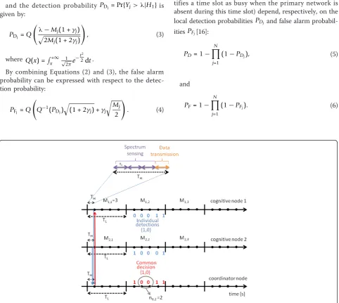
As illustrated on Figure 1, we consider that everyTH seconds, each node sends a one bit value representing the local hard decision about the primary network presence to the base station. The base station combines the received bits in order to make a global decision for the nodes. The base station decision is sent back to the node as a one bit value. The duration of the communication with the base station is assumed to be negligible compared to the dura-tionTHof a time slot. In this article, we focus on the logi-cal-OR fusion rule at the base station but the other fusion rules could be similarly analyzed. Under the logical-OR fusion rule, the global detection probabilityPD(defined as the probability that the coordinator node identifies a time slot as busy when the primary network is present during this time slot) and the global false alarm probabilityPF (defined as the probability that the coordinator node iden-tifies a time slot as busy when the primary network is absent during this time slot) depend, respectively, on the local detection probabilities PDj and false alarm probabil-itiesPFj[16]:
PD= 1− N
j=1
(1−PDj), (5)
and
PF = 1− N
j=1
(1−PFj). (6)
Given a target global detection probability P¯D, we thus have:
PDj = 1−(1− ¯PD)
1/N
, (7)
and Equation (4) can be rewritten as:
PFj=Q
2.2. Throughput of a secondary user
The random variable representing the presence of the primary network in each time slotnis denotedH(n) (H
(n) Î {H0, H1}) and is assumed to be a Markov Chain
characterized by a transition matrix [puv]. It is assumed that the probabilityp01of the primary network
appari-tion is small compared to the probability p00. As a
result, the secondary users can decide to communicate or not during a time slot based on the result of their sensing in the previous time slot while limiting the probability of interference with the primary network.
A secondary user performs data transmission during the time slots that have been identified as free by the base sta-tion. In each of these time slots,MjTSseconds are used by the secondary user to sense the spectrum, where TS denotes the sampling period. The remainingTH- MjTS seconds are used for data transmission. The secondary user average throughputRjis given by the sum of the through-put obtained when the primary network is absent and no false alarm has been generated by the base station plus the throughput obtained when the primary network is present but has not been detected by the base station [6]:
Rj=
ary probability of the primary network absence, CH0,j
represents the data rate of the secondary user underH0
and CH1,j represents the data rate of the secondary user
under H1. The target detection probability P¯D is required to be close to 1 since the cognitive radios should not interfere with the primary network; more-over, πH0 is usually close to 1, CH1,jCH0,j due to the
interference from the primary network [6] and it is
assumed that p00≥ p10. Therefore, (9) can be
approxi-mated by:
Rj≈
TH−MjTS
TH π
H0(1−PF)p00CH0,j (10)
2.3. Sensing time allocation problem
Equations (6), (8), and (10) show that there is a tradeoff for the choice of the sensing window lengthMj: on the one hand, if Mj is high then the user j will not have enough time to perform his data transmission and Rj will be low. On the other hand, if all the users use low
Mjvalues, then the global false alarm probability in (10) will be high and all the average throughputs will be low.
The sensing time allocation problem consists in find-ing the optimal sensfind-ing window length {M1, . . .,MN} that minimize a cost functionf(R1, . . .,RN) depending on the secondary throughputs.
In this article, the following cost function is consid-ered:
where R¯j denotes the throughput required by nodej. It is observed that the cost decreases with respect to
RjuntilRjreaches the threshold value R¯j, then the cost increases with respect to Rj. This should prevent sec-ondary users from selfishly transmitting with a through-put higher than required, which would reduce the achievable throughputs for the other secondary users.
Although a base station could determine the sensing window lengths that minimize function (11) and send these optimal values to each secondary user, in this arti-cle we rely on the secondary users themselves to deter-mine their individual best sensing window length. This decentralized allocation avoids the introduction of sig-naling overhead in the system.
3. Power allocation problem formulation
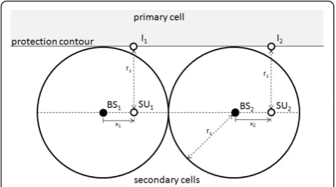
We consider a large circular primary cell made up of one central primary emitter and several primary recei-vers whose positions are unknown. The primary emitter could be a DTV broadcasting station that communicates with multiple passive receivers.
The secondary network uses the same frequency band as the primary network and consists inL adjacent sec-ondary cells. Each secsec-ondary cell is made up of one cen-tral secondary base station and multiple secondary users. For the sake of simplicity, all the secondary users (SU) are assumed to be located on the line that joins the L
is referred to [10] for more realistic assumptions regard-ing the geometry of the power allocation problem.
In order to protect the primary receivers from receiv-ing harmful interference from the secondary users, a
protection contour is defined around the primary emitter as a circle on which the received primary SINR must be superior to a given threshold SINRpTh. The secondary cells are located around the protection contour. As the primary cell ray is assumed to be much larger than the secondary cells ray, the protection contour can be approximated by a line parallel to the secondary base stations line.
The secondary network is assumed to follow a Time Division Multiple Access (TDMA) scheme, so that at each time only one secondary user SUl communicates with its base station BSlin cell l(l Î {1, . . ., L}). The difference between SUland BSl abscissa is denotedxl. The point on the protection contour whose distance with SUlis minimal is denotedIl. We assume that each celll deploys sensors on the protection contour so that it is able to measure the primary network SINR at the pointIl, denoted SINR
p l.
In this article, the analysis is focused on the interfer-ence generated by the upstream transmissions of the secondary users. It is assumed that the secondary SINR at each base station l, denoted SINRs
l, needs to be superior to a given threshold SINRs
Th for the secondary
communication to be reliable.
The power allocation problem consists in finding the optimal secondary users transmission powers {P1, . . ., PL} that minimize a cost function f
SINRs1,. . ., SINRsL depending on the secondary SINRs, under the con-straints that
SINRpl ≥SINRpTh ∀l∈ {1,. . .,L} (12)
In this article, the following cost function is consid-ered:
It is observed that the cost decreases with respect to SINRs
l until SINRsl reaches the threshold value SINRsTh,
then the cost increases with respect to SINRsl. This should prevent secondary users from selfishly transmit-ting with a power higher than required, which would remove transmission opportunities for other secondary users.
The primary SINRs in Equation (12) are given by:
SINRpl = P
p
σ2 + L
k=1PkhSUIl k
wherePpis the power that is received on the protec-tion contour from the primary transmitter, s2 is the noise power and hSUk
Il is the link gain between SUkand the pointIlon the protection contour.
The secondary SINRs in Equation (13) are given by:
SINRsl = Plh In this article, we consider free space path loss. There-fore, the link gains are computed as follows:
hSUk transmission frequency and c is the speed of light in vacuum.
4. Learning algorithm 4.1. Q-learning algorithm
In this article, we use two multi-agent Q-learning algo-rithms. The first one is used to allocate the secondary user sensing times and the second one is used to allo-cate the secondary user transmission powers. In the sen-sing time allocation algorithm, each secondary user is an agent that aims to learn an optimal sensing time alloca-tion policy for itself. In the power allocaalloca-tion algorithm, each secondary base station is an agent that aims to learn an optimal power allocation policy for its cell.
Q-learning implementation requires the environment to be modeled as a finite-state discrete-time stochastic Figure 2Primary and secondary networks whenL= 2 adjacent
system. The set of all possible states of the environment is denoted S. At each learning iteration, the agent that executes the learning algorithm performs an action cho-sen from the finite set A of all possible actions. Each learning iteration consists in the following sequence:
1) The agent senses the state s∈S of the environment
2) Based on s and its accumulated knowledge, the agent chooses and performs an action a∈A. 3) Because of the performed action, the state of the environment is modified. The new state is denoted s’ The transition from s tos’generates a cost c Î ℝ
for the agent.
4) The agent uses c and s’ to update the accumu-lated knowledge that made him choose the action a
when the environment was in states.
The Q-learning algorithm keeps a quality information (the Q-value) for every state-action couple (s, a) it has tried. The Q-value Qi(s, a) represents how high the expected quality of an actionais when the environment is in state s [17]. The following policy is used for the selection of the actionaby the agent when the environ-ment is in states:
a=
arg max
˜
a∈A Q(s,a˜), with probability 1− random action∈A, with probability (16)
where is the randomness for exploration of the learning algorithm.
The cost c and the new state s’ generated by the choice of action ain states are used to update the Q-valueQ(s, a) based on how good the action awas and how good the new optimal action will be in states’. The update is handled by the following rule:
Q(s,a)←(1−α)Q(s,a) +α(−c+γmax a∈AQ(s
,a))
(17)
whereais the learning rate andgis the discount rate of the algorithm.
The learning ratea Î[0, 1] is used to control the lin-ear blend between the previously accumulated knowl-edge about the (s, a) couple, Q(s, a), and the newly received quality information −c+γmaxa∈AQ(s,a). A high value of a gives little importance to previous experience, while a low value of agives an algorithm that learns slowly as the stored Q-values are easily altered by new information.
The discount rateg Î [0, 1] is used to control how much the success of a later actiona’should be brought back to the earlier action athat led to the choice of a’. A high value ofggives a low importance to the cost of
the current action compared to the Q-value of the new state this actions leads to, while a low value of gwould rate the current action almost only based on the immediate reward it provides.
The randomness for exploration Î[0, 1] is used to control how often the algorithm should take a random action instead of the best action it knows. A high value offavors exploration of new good actions over exploi-tation of existing knowledge, while a low value of rein-forces what the algorithm already knows instead of trying to find new better actions. The exploration-exploitation trade-off is typical of learning algorithms. In this article, we consider online learning (i.e., at every time step the agents should display intelligent behaviors) which requires a lowvalue.
4.2. Q-Learning implementation for sensing time allocation
Each secondary user is an agent in charge of sensing the environment state, selecting an action according to pol-icy (16), performing this action, sensing the resulting new environment state, computing the induced cost and updating the state-action Q-value according to rule (17). In this section, we specify the states, actions and cost function used to solve the sensing time allocation problem.
At each iteration tÎ {1, . . .,K} of the learning algo-rithm, a secondary user jÎ {1, . . ., N} represents the local statesj, tof the environment as follows:
sj,t =nH0,t−1 (18)
where nH0,t−1 denotes the number of time slots that
have been identified as free by the base station during the (t-1)th learning period.
The number of free time slots takes one out of r
values:
nH0,t ∈ {0, 1,. . .,r}.
At each iterationt, the action selected by the second-ary userjis the durationMj, tof the sensing window to be used during the TLseconds of the learning iteration
t. It is assumed that one learning iteration spans several time slots:
TL=rTH,r∈N0.
The optimal value ofr will be determined in Section 5. Letsdenotes the ratio between the duration of a time slot and the sampling period:
TH=sTS,s∈N0,
Mj,t∈ {0, 1,. . .,s}. (19)
In this article, we compare the performances of the sensing time allocation system for two different cost functionscj, t. We firstly define acompetitive cost
func-tionin which the cost decreases if the average through-put realized by nodejincreases:
cj,t =− ˆRj,t (20)
where Rˆj,t denotes the average throughput Rˆj,t rea-lized by nodejduring the learning periodt:
ˆ
With this cost function, every node tries to achieve the maximum Rˆj,t with no consideration for the other nodes in the secondary network. We secondly define a
cooperative cost function in which the cost decreases if the difference between the realized average throughput and the required average throughput decreases:
cj,t= (Rˆj,t− ¯Rj)2 (23)
This last cost function penalizes the actions that lead to a realized average throughput that is higher than required, which should help the disadvantaged nodes (i. e., the nodes that have a low data rate CH0,j) to achieve
the required average throughput.
4.3. Q-Learning implementation for distributed power allocation
Each secondary BS is an agent in charge of sensing the environment state, selecting an action according to pol-icy (16), performing this action, sensing the resulting new environment state, computing the induced cost and updating the state-action Q-value according to rule (17). In this section, we specify the states, actions, and cost function used to solve the power allocation problem.
At each iteration tÎ {1, . . .,K} of the learning algo-rithm, a base stationlÎ {1, . . ., L} represents the local statesl, tof the environment as the following triplet:
sl,t={xl,t,Pl,t,Il,t} (24)
where xl, t is the local coordinate of the currently transmitting secondary user SUl,Pl, tis the power cur-rently allocated to this user and Il, tÎ {0, 1} is a binary indicator that specifies whether the measured aggre-gated interference at the sensor Il on the protection
contour is above or below the acceptable threshold. It is defined as:
Il,t=
1 if SINRpl,t<SINRpTh
0 otherwise (25)
For Q-learning implementation the states have to be quantized. Therefore it is assumed that xl, t takes one out of the followingξvalues:
xl,t∈
Similarly,Pl, ttakes one out of the followingjvalues:
Pl,t∈=
wherePminandPmaxare the minimum and maximum
effective radiated powers (ERP) in dBm.
At each iterationt, the action selected by the base sta-tion BSlis the power to allocate to the currently trans-mitting secondary user SUl. The set of all possible actions is therefore given by Equation (27).
In this article, we compare the performances of the power allocation system for two different cost functions
cl, t. We first define a competitive cost functionin which the cost decreases if the secondary SINR at the base sta-tion increases, provided that the aggregated interference generated on the primary protection contour does not exceeds the acceptable level:
cl,t=
−SINRsl,t if SINRpl,t≥SINRpTh
+∞ otherwise (28)
where +∞represents a positive constant that is chosen large enough compared to SINRsl,t. With this cost func-tion, every agent tries to achieve the maximum SINRs l with no consideration for the other secondary cells in the network. Second, we define a cooperative cost func-tion in which the cost decreases if the difference between the secondary SINR at the base station and the required secondary SINR threshold decreases, provided that the aggregated interference on the protection con-tour is acceptable:
where +∞represents a positive constant that is chosen large enough compared to (SINRsl,t−SINRsTh)2. This
the aggregated interference Nk=1,k=lPkhSUBSlk is high) to achieve the required secondary SINR threshold.
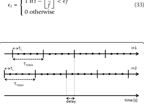
In this article, the impact of the frequency of the learning algorithm is also analyzed. If TTDMA denotes
the length of a TDMA time slot and TL denotes the length of a learning iteration, then
f = TTDMA
TL
(30)
indicates how many times a learning loop is executed during one TDMA time slot (i.e., for a fixed secondary transmitter SUlin celll). It is assumed that every second-ary cell uses the same TDMA time slot lengthTTDMAas
well as the same learning iteration lengthTL. However, the secondary transmissions as well as the learning itera-tions are assumed asynchronous, as illustrated on Figure 3. Finally, three exploration strategies are compared in this article. These three exploration strategies are char-acterized by the same average randomness for explora-tion ¯.
The first exploration strategy consists in using a con-stantparameter during theKlearning iterations:
t=¯ (31)
In the second exploration strategy,decreases linearly between the values t=1= 2¯ and t=K= 0:
t= 2¯
K−t K−1
(32)
In the third exploration strategy, the algorithm does pure exploration during the ¯f first learning iterations of each TDMA time slot, then pure exploitation during the remaining (1− ¯)f last learning iterations of the time slot (see, Figure 4):
t =
⎧ ⎨ ⎩
1 ift−
t f
<¯f
0 otherwise
(33)
Note that for both the sensing time and power alloca-tion problems, the agents have an imperfect knowledge of the state of the environment. The state represented by an agent at each iteration of the Q-learning algo-rithm is actually an imperfect estimation of the environ-ment state. In this case, the convergence demonstration of single agent Q-learning [18] does not hold. However, multi-agent Q-learning algorithms have been success-fully applied in multiple scenarios [11] and in particular to cognitive radios [10,12,19]. Numerical results will show that both Q-learning algorithms presented in this article converge as well.
5. Numerical results
5.1. Sensing time allocation algorithm
Unless otherwise specified, the following simulation parameters are used: we consider N= 2 nodes able to transmit at a maximum data rate CH0,1=CH0,2= 0.6.
They each require a data rate R¯1=R¯2= 0.1. One node
has a sensing channel characterized by g1 = 0 dB and
the second one has a poorer sensing channel character-ized byg2= -10 dB.
It is assumed that the primary network transition probabilities arep00 = 0.9,p01= 0.1,p10 = 0.2, andp11
= 0.8. The target detection probability is P¯D= 0.95. We considers = 10 samples per time slot andr= 100 time slots per learning periods. The Q-learning algo-rithm is implemented with a learning ratea= 0.5 and a discount rate g= 0.7. The chosen exploration strategy consists in using = 0.1 during the firstK/2 iterations and then= 0 during the remainingK/2 iterations.
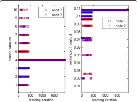
Figure 5 gives the result of the Q-learning algorithms when no exploration strategy is used ( = 0). It is observed that after 430 iterations, the algorithm con-verges toM1 =M2= 4 which is a sub-optimal solution.
The optimal solution obtained by minimizing Equation (11) isM1 = 4, M2 = 1 (as the second node has a low
sensing SNR, the first node has to contribute more to the sensing of the primary signal). After convergence,
the normalized average throughputs are
ˆ
R2,opt/CH0,2= 0.144 whereas the optimal normalized
Figure 3The transmissions and the learning iterations in the multiple secondary cells are assumed asynchronous.
Figure 4Exploration strategy that consists in doing pure exploration during the ¯TTDMA first seconds of each TDMA time slot, then pure exploitation during the remaining
average throughputs are Rˆ1,opt/CH0,1= 0.096 and
ˆ
R2,opt/CH0,2= 0.144 and lead to an inferior global cost
in Equation (11).
Figure 6 gives the result of the Q-learning algorithms when the exploration strategy described at the beginning of this Section is used. It is observed that the algorithm converges to the optimal solution defined in the pre-vious paragraph.
Table 1 compares the performance of the sensing time allocation algorithm implementation based on the coop-erative cost function defined by Equation (23) with the one based on the competitive cost function defined by Equation (20). The cooperative cost function penalizes the actions that lead to a higher than required through-put and as a result performs better (i.e., gives higher realized average throughputs Rˆj) than the competitive
cost function, in different scenarios. In particular, it helps achieve fairness among the nodes when one of the nodes has a lower sensing SNR (in which case the other nodes tend to contribute more to the sensing) or when one of the nodes has an inferior channel capacity (in which case this node tends to contribute less to the sing). The data in Table 1 are the averages of the sen-sing window lengths and realized throughputs obtained in each scenario.
Figure 7 shows the average normalized throughput that is obtained with the algorithm with respect to para-meterr = TL/TH when the total duration of execution of the algorithm, equal to rK TH , is kept constant. When r decreases, then the learning algorithm is
exe-cuted more often but the ratio nH0,t
r becomes a less
accurate approximation of πH0(1−PF)p00 and as a
result, the agent becomes less aware of its impact on the false alarm probability. Therefore, there is a tradeoff value forraround r≈10 as illustrated on Figure 7.
After convergence of the algorithm, if the value of the local SNR g1 decreases from 0 dB to -10 dB, the
algo-rithm requires an average of 1200 iterations before con-verging to the new optimal solution M1 = M2 = 1.
According to Equation (17), each Q-learning iteration requires four additions and five multiplications per node. This result can be compared with the complexity of the centralized allocation algorithm which must be solved numerically. By using a constant step gradient descent optimization algorithm to solve the centralized allocation problem, it was measured that the conver-gence occurred after an average of four iterations. At each iteration of the algorithm, the partial derivatives of the cost function with respect to the sensing times are evaluated. It can be shown that 18N -1 multiplications and 8N -1 additions are needed for this evaluation. As a result, the centralized allocation algorithm will have a lower computational complexity per node than the learning algorithm. The main advantage of the Q-Figure 5 Result of the Q-learning algorithm when no
exploration strategy is used (= 0).
Figure 6 Result of the Q-learning algorithm when an exploration strategy is used (≠0).
Table 1 Average sensing window lengths and realized throughputs obtained with the competitive and cooperative cost functions
CH0,1= 0.6 CH0,1= 0.6 CH0,1= 1.0
CH0,2= 0.6 CH0,2= 0.6 CH0,2= 0.2
g1= -5dB g1=0dB g1= -5dB
g2= -5dB g2= -10dB g2= -5dB
Competitive
M1 M2 2.3 2.0 3.3 0.67 2.5 2 ˆ
R1 Rˆ2 0.0378 0.0397 0.0556 0.0780 0.0635 0.0133
Cooperative
M1 M2 3.8 3.7 3.7 1.8 3.3 2.3 ˆ
learning algorithm is therefore the minimization of con-trol information sent between the secondary nodes and the coordinator node.
5.2. Power allocation algorithm
The performance of the Q-learning algorithm presented in Section 4 is evaluated by comparison with the opti-mal centralized power allocation scheme in which a base station having a perfect knowledge of the environ-ment chooses the optimal transmission powers each time there is a change in the environment (i.e., when-ever a TDMA time slot ends in any of theLcells). The optimal allocated powers are determined by selecting the transmission powers (P1, . . .,PL) ÎΨL that maxi-mize Equation (13) under the constraints given in Equa-tion (12).
The learning algorithm performance metrics consid-ered here is the distancedt(in dB) between the second-ary SINRs obtained with the multi-agent Q-learning algorithm and the secondary SINRs given by the optimal allocation algorithm:
dt=
N
l=1
SINRs
t,l−SINR s t,l
2
t∈ {1,. . .,K} (34)
where SINRst,l denotes the secondary SINR measured at iterationtat BSlin the distributed learning scenario and SINRst,l denotes the secondary SINR measured at iterationtat BSlin the optimal centralized scenario.
The performance is evaluated for L = 2 secondary cells with a ray rs = 15 km. The received power from the primary emitter on the protection contour is Pp= 0 dBm. Both the primary and the secondary network use a frequency fc = 2.45 GHz. The minimum acceptable
primary SINR on the protection contour is
SINRpTh= 20 dB. The desired secondary SINR at the base stations is SINRsTh= 3 dB. The secondary users are
allocated powers ranging from Pmin = 0 dBm to
Pmax=
1
hSUl Il
−σ2+ Pp
SINRpTh
= 66.4 dBm.
The secondary transmission powersPl, tare quantized on j= 15 levels and the local coordinates xl, t of the secondary users are quantized onξ = 10 levels. The Q-learning algorithm is implemented with a Q-learning rate a= 0.5, a discount rate g= 0.9 and an average random-ness for exploration ¯= 0.1.
Figure 8 compares the performance of the power allo-cation algorithm implementation based on the coopera-tive cost function defined by Equation (29) with the one based on the competitive cost function defined by Equa-tion (28). The cooperative cost funcEqua-tion penalizes the actions that lead to a higher than required secondary SINR and as a result performs better (i.e., gives a lower distancedtto the optimal solution) than the competitive cost function.
Figure 9 compares the convergence speed of the Q-learning algorithms when different Q-learning frequenciesf
are used. The Q-learning algorithm converges faster when f increases but the improvement is negligible whenf > 50. After about 20000 TDMA time slots, the performance of the algorithm is constant and does not depend on the learning frequency.
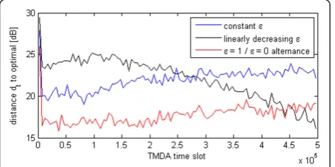
Figure 10 compares performance of the Q-learning algorithms when different exploration policies are used. The linearly decreasing strategy defined by Equation (32) converges more slowly than the two other analyzed strategies but leads to better final results. The averagedt of this strategy, computed on the last 50,000 time slots, is equal to 17.5 dB. The full exploration/full exploitation alternance strategy defined by Equation (33) is the strat-egy that gives the best initial performance but leads to final results that are inferior to those obtained with the linearly decreasing . The averagedt, computed on the Figure 7Average throughput achieved by the Q-learning
algorithm with respect to parameter r= TL TH.
Figure 8Distancedtbetween the secondary SINRs generated
last 50,000 time slots, is equal to 18.7 dB. The perfor-mance of the constant strategy defined by Equation (31) is always inferior to the performance of the alter-nance strategy. The average dt, computed on the last 50,000 time slots, is equal to 23.0 dB.
The complexity of the decentralized power allocation Q-learning algorithm can be compared to a reference gradient descent centralized power allocation algorithm, similarly to the analysis performed in Section 1. The conclusion is the same as for the sensing time allocation algorithm: the centralized allocation algorithm has a lower computational complexity than the decentralized Q-learning algorithm whose main advantage is therefore that the base stations do not need to exchange control information.
6. Conclusion
In this article, we have proposed two decentralized Q-learning algorithms. The first one was used to solve the problem of the allocation of the sensing durations in a cooperative cognitive network in a way that maximize the throughputs of the cognitive radios. The second one
was used to solve the problem of power allocation in a secondary network made up of several independent cells, given strict limit for the allowed aggregated inter-ference on the primary network. Compared to a centra-lized allocation system, a decentracentra-lized allocation system is more robust, scalable, maintainable and computation-ally efficient.
Numerical results have demonstrated the need for an exploration strategy for the convergence of the sensing time allocation algorithm. It has also been observed that the strategy of keeping the exploration parameter con-stant in the power allocation algorithm is less efficient than using a linearly decreasing parameter or imple-menting an alternance between full exploration and full exploitation, this latest exploration policy leading to the fastest convergence of the power allocation algorithm.
It has furthermore been shown that the implementa-tion of a cost funcimplementa-tion that penalizes the acimplementa-tions leading to a higher than required throughput in the sensing time allocation algorithm gives better results than the implementation of a cost function without such penalty. Similarly, the implementation of a cost function that penalizes the actions leading to a higher than required secondary SINR in the power allocation algorithm gives better results than the implementation of a cost function without such penalty.
Finally, it has been shown that there is an optimal tra-deoff value for the frequency of execution of the sensing time allocation algorithm. The power allocation algo-rithm has been shown to converge faster when its fre-quency of execution increases, until the frefre-quency reaches an upper bound where the increase of the con-vergence speed gets insignificant.
Competing interests
The authors declare that they have no competing interests.
Received: 20 May 2011 Accepted: 10 April 2012 Published: 10 April 2012
References
1. FK Jondral, TA Weiss, Spectrum pooling: An innovative strategy for the enhancement of spectrum efficiency. IEEE Radio Commun.42(3), S8–S14 (2004)
2. B Aazhang, A Sendonaris, E Erkip, User cooperation diversity. Part I: system description IEEE Trans Commun.51(11), 1927–1938 (2003)
3. GB Bazerque, JA Giannakis, Distributed spectrum sensing for cognitive radio networks by exploiting sparsity. IEEE Trans Signal Process.58(3), 1847–1862 (2010)
4. E Peh, Y-C Liang, Y Zeng, AT Hoang, Sensing-throughput tradeoff for cognitive radio networks, IEEE Trans. Wirel Commun.4(7), 1326–1337 (2008) 5. S Stotas, A Nallanathan, Sensing time and power allocation optimization in
wideband cognitive radio networks, inGLOBECOM 2010, 2010 IEEE Global Telecommunications Conference, Miami, pp. 1–5 (2010)
6. W Beibei, KJR Liu, TC Clancy, Evolutionary cooperative spectrum sensing game: how to collaborate? IEEE Trans. Commun.58(3), 890–900 (2010) 7. S Shankar, C Cordeiro, Analysis of aggregated interference at DTV receivers
in TV bands, inProceedings of the 3rd International Conference on Cognitive Radio Oriented Wireless Networks and Communications (CrownCom), Singapore, pp. 1–6 (2008)
Figure 9Distancedtbetween the secondary SINRs generated
by the Q-learning algorithm and the optimal secondary SINRs when using different frequencies of learningfin the Q-learning implementation. The randomness of explorationis constant and a cooperative cost function is used.
Figure 10Distancedtbetween the secondary SINRs generated
8. R Tandra, SJ Shellhammer, S Shankar, J Tomcik, Performance of power detector sensors of DTV signals in IEEE 802.22 wrans, inProceedings of First International Workshop on Technology and Policy for Accessing Spectrum, Boston, (2006)
9. A Dejonghe, A Bahai, LV der Perre, M Timmers, S Pollin, F Catthoor, Accumulative interference modeling for cognitive radios with distributed channel access, inProceedings of the 3rd International Conference on Cognitive Radio Oriented Wireless Networks and Communications (CrownCom), Singapore, pp. 1–7 (2008)
10. A Galindo-Serrano, L Giupponi, Distributed q-learning for aggregated interference control in cognitive radio networks. IEEE Trans Veh Technol.59, 1823–1834 (2010)
11. P Liviu, L Sean, Cooperative multi-agent learning: the state of the art, Auton. Agents Multi-Agent Syst.11(3), 387–434 (2005)
12. H Li, Multi-agent Q-learning for competitive spectrum access in cognitive radio systems, in5th IEEE Workshop on Networking Technologies for Software Defined Radio Networks, pp. 1–6 (2010)
13. H Urkowitz, Energy detection of unknown deterministic signals, in
Proceedings of the IEEE.vol 55, 523–531 (1967)
14. FF Digham, M-S Alouini, MK Simon, On the energy detection of unknown signals over fading channels. IEEE Trans Commun.55(1), 21–24 (2007) 15. J Ma, G Zhao, Y Li, Soft combination and detection for cooperative
spectrum sensing in cognitive radio networks. IEEE Trans Wirel Commun. 7(11), 4502–4507 (2008)
16. Y-C Liang, Y Zeng, ECY Peh, AT Hoang, Sensing-throughput tradeoff for cognitive radio networks. IEEE Trans Wirel Commun.7(4), 1326–1337 (2008) 17. I Millington,Artificial Intelligence for Games, (Morgan Kaufmann Publishers,
San Fransisco, CA, 2006), pp. 612–628
18. C Watkins, P Dayan, Technical note: Q-learning. Mach Learn.8, 279–292 (1992). doi:10.1023/A:1022676722315
19. C Wu, K Chowdhury, M Di Felice, W Meleis, Spectrum management of cognitive radio using multi-agent reinforcement learning, inProceedings of the 9th International Conference on Autonomous Agents and Multiagent Systems: Industry track, AAMAS’10, (International Foundation for Autonomous Agents and Multiagent Systems), Richland, SC, pp. 1705–1712 (2010)
doi:10.1186/1687-1499-2012-138
Cite this article as:van den Biggelaaret al.:Sensing time and power allocation for cognitive radios using distributed Q-learning.EURASIP Journal on Wireless Communications
and Networking20122012:138.
Submit your manuscript to a
journal and benefi t from:
7Convenient online submission 7Rigorous peer review
7Immediate publication on acceptance 7Open access: articles freely available online 7High visibility within the fi eld
7Retaining the copyright to your article