DISCRETE ELEMENT ANALYSIS OF SLOPE COLLAPSE BEHAVIOR
TRIGGERED BY AN EARTHQAKE GENERATION AROUND NUCLEAR
POWER PLANTS AND ITS APPLICABILITY
Hitoshi Nakase 1, Guoqiang Cao2, Hitoshi Tochigi3, and Takashi Matsushima4
1
Doctor of Civil Engineering, Specialist, Civil Engineering Center, Tokyo Electric Power Services Co., Ltd., Japan 2
Doctor of Civil Engineering, Nuclear & Engineering Department, ITOCHU Techno-Solutions Corporation, Japan 3
Doctor of Civil Engineering, Civil Engineering Research Laboratory, Central Research Institute of Electric Power Industry, Japan 4
Doctor of Civil Engineering, Professor of Department of Engineering Mechanics and Energy, University of Tsukuba, Japan
ABSTRACT
Risk evaluation of slope failure against nuclear power plants, which is induced by unexpectedly large earthquakes, has been urgent need for disaster prevention measures. Specially, for risk evaluation of slope failure, understanding of information such as traveling distances, collision velocities, and collision energies is very important. Discrete Element Method (DEM) such as particle simulation method contributes important role on predicting the detailed behaviour of slope failure physics. In this study, instead of accurately predicting the complicated behaviour of sliding and falling for each rock, we introduce the DEM modelling to evaluate the average traveling distance of collapsed rocks and its statistical variability. We conduct the validation test of the proposed DEM model on the basis of reconstruction of experiment results. Finally, validity of the proposed method is evaluated and its applicability and technical assignments are also discussed
INTRODUCTION
In the process of risk evaluation of against nuclear power stations and related facilities in these days, they are required to evaluate the effects of slope collapse and rock fall from unexpectedly large earthquakes on the important infrastructures. For those evaluations, we think that the discrete element method (hereafter called as DEM, Cundall(1979)) is one of effective numerical approaches.
However, for analysing rock collision problem, the slight difference in collision angle tends to significantly affect the rock kinematics after collision. Therefore, despite of accurately modelling the rock geometry, it is difficult to deterministically evaluate the propagation natures (path, velocity, and traveling distance) of collision process. In addition, because a realistic slope and nature of subsurface structure are very complex and variable, deterministically evaluation is even more difficult. Because of that, traveling distance of a rock mass falling down along the slope is usually estimated on the basis of probability distribution.
behaviour of a single collision, the analysis is thought to be good enough for probabilistic evaluation of rock falling.
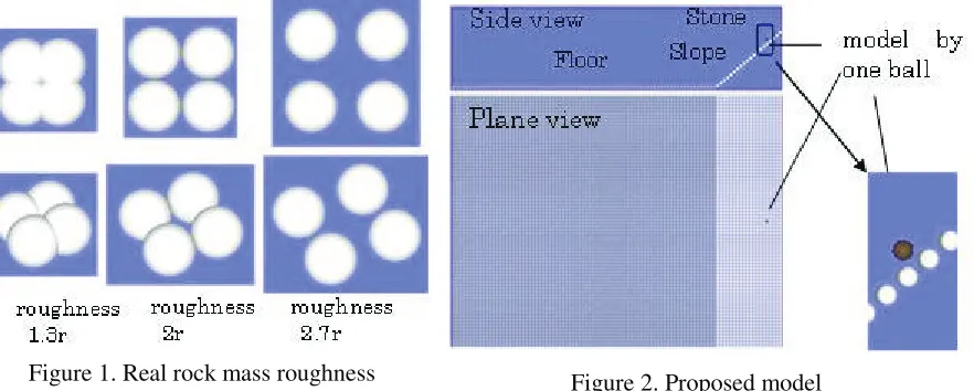
Based on this assumption, in this study we evaluate the validity of simplifying geometry of rock mass in which rock mass is expressed by a single ball, and parameters to express slope roughness are discussed. And, we compare the result of analysis with the rock-fall experiments and validity is evaluated.
DEM MODELING PROCEDURE
Modelling concept
Without modelling the shape of the rock mass, the rock mass is modelled by one ball. The roughness of the rock shape is expressed by spacing balls of same radius on the slope or the floor in the equal interval as shown in Figure 1(left) and in Figure 2. Here, roughness 2r means that the ball interval is two times as large as the radius of the ball.
Namely, when the rock mass drops to the floor as shown in Figure 3, the irregular bounce is expressed by the impaction in spherical surfaces and bounce irregularly. For the convenience, this model is named simple model.
Restitution coefficient
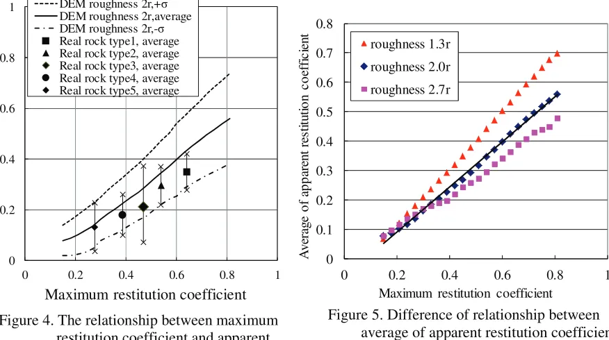
The restitution coefficient is the most important factor in rock fall simulations of this study. Figure 4 shows comparisons of results of the real rock mass and the simple model. Here, maximum restitution coefficient means the result obtained from experiment with a nearly sphere rock and from the simple model with a ball falling to the top of fixed ball. Apparent restitution coefficient means an average value in a set of measurements (Vn’/Vn, the ratio of vertical velocities of Figure 3(left)) in experiments. In the simple model it is an average value in a set of calculated values (Vn’/Vn, the ratio of vertical velocities of Figure 3(right)) by falling the ball from different horizontal positions. The results of the range of
fluctuation with ! " by DEM simple model is shown by the long dashes lines, respectively. The experimental results are shown by the extending lines. Here, the floor is modeled by spacing the balls at the equal interval in the simple model, corresponding to roughness 2r in Figure 1 (left).
It seems that DEM result is close to the experiment results. However, in comparison with the experimental results, fluctuation increases when both maximum and apparent restitution coefficient increase. This difference with the experimental results can be decreased by changing the ball interval for
Figure 1. Real rock mass roughness
modelling the floor in the simple model. Figure 5 shows the results obtained from the simple model. Apparent restitution coefficient decreases when the ball interval increases.
Figure 3. Irregular bounces of a real rock mass and expression by the impaction in spherical surface and bounce irregularly 0 0.2 0.4 0.6 0.8 1
0 0.2 0.4 0.6 0.8 1
A p p a re n t re st it u ti o n c o e ffi c ie n t
Maximum restitution coefficient DEM roughness 2r,+ı
DEM roughness 2r,average DEM roughness 2r,-ı
Real rock type1, average Real rock type2, average Real rock type3, average Real rock type4, average Real rock type5, average
0 0.1 0.2 0.3 0.4 0.5 0.6 0.7 0.8
0 0.2 0.4 0.6 0.8 1
A v er ag e o f ap p ar en t re st it u ti o n c o ef fi c ie n t
Maximum restitution coefficient roughness 1.3r
roughness 2.0r roughness 2.7r
NUMERICAL REPRESENTATION OF ROCK DROP TEST
Single rock drop test
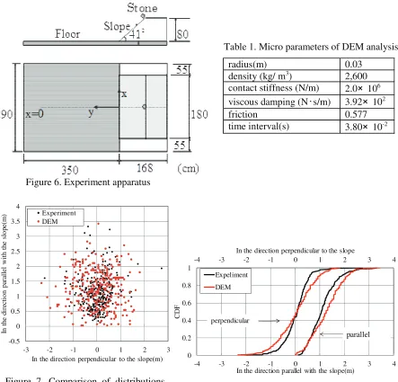
Tochigi(2010) conducted experiments by dropping one and more stones (limestone) with the diameters of 40-80mm. In single rock drop test shown in Figure.6, 300 stones were dropped under gravity one by one, and all arrival distances of stones were measured. In the experiment, each stone placed on the top of the slope along the long length was slowly put out by a finger to be fallen down and removed out after it stopped on the floor. All stones almost did not slip straight to the floor and begun to rotate after slipped centimeters along the slope.
Figure 4. The relationship between maximum restitution coefficient and apparent restitution coefficient surface and bounce
irregularly
Figure 5. Difference of relationship between average of apparent restitution coefficient
The parameters and the analysis conditions of DEM are shown in Table 1. The density is assigned same as experimental stone. The contact stiffness and friction are assigned as in Tochigi(2010). The viscous damping coefficient between the stone and the concrete plate is assigned property corresponding to an estimated maximum restitution coefficient 0.48 studied in the separated part. Here, the normal and shear stiffness and viscous damping coefficient are assumed to be equal. Here, the initial positions of 300 stones are randomly placed within a square with the side equal to the diameter of stone model to vary the reached positions. The distance of ball interval on the slope and bottom are same as the diameter (roughness 2r shown in Figure.5).
Figure.7 compares the distribution of stopped positions of stones in the experiment and the simple model. The results of the simple model approximately correspond to the experiment.
Figure.8 compares the results of cumulative distribution probability in the direction perpendicular to the slope (expanse distance) and in the direction parallel with the slope (arrival distance), respectively. Nonetheless the simple model has a little bit large fluctuation in the expanse distance, the average behaviour is approximately same as experiment. It may be said that the simple model evaluates the experiment on the safe side, anyway.
radius(m) 0.03
density (kg/ m3) 2,600
contact stiffness (N/m) 2.0# 106
viscous damping (N$s/m) 3.92# 102
friction 0.577
time interval(s) 3.80# 10-2
-0.5 0 0.5 1 1.5 2 2.5 3 3.5 4
-3 -2 -1 0 1 2 3
In
t
h
e
d
ir
ec
ti
o
n
p
ar
al
le
l
w
it
h
t
h
e
sl
o
p
e(
m
)
In the direction perpendicular to the slope(m) Experiment
DEM
-4 -3 -2 -1 0 1 2 3 4
0 0.2 0.4 0.6 0.8 1
-4 -3 -2 -1 0 1 2 3 4
In the direction perpendicular to the slope
C
D
F
In the direction parallel with the slope(m) Expeliment
DEM
perpendicular
parallel Figure 6. Experiment apparatus
Table 1. Micro parameters of DEM analysis.
Figure 7. Comparison of distributions of stopped rock positions by experiment and simulation
Collapse test of rocks
Next, we performed the simulation for collapse test of rocks by using the simple model. The experiment is shown in Figue.9 in which rocks were deposited in a box and collapsed by moving the wall of the box suddenly. The arrival positions of rocks ware measured. Rocks used in the experiment were 50 kg.
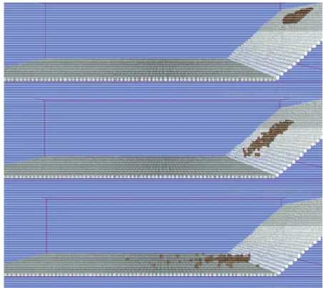
The particle number in this simulation is 177. The restitution coefficient of particles is assumed as 0.48. The snap shots of the simulation results are shown in Figure 10.
Figure 11 compares the distributions of stopped rock positions by the experiment and the simulation on the simple model and it seems that the results are similar. And the comparison of the cumulative distributions of stopped rock positions is shown in Figure 12. The simulation accords with the experiment.
-0.5 0 0.5 1 1.5 2 2.5 3
-3 -2 -1 0 1 2 3
In
t
h
e
d
ir
ec
ti
o
n
p
ar
al
le
l
w
it
h
t
h
e
sl
o
p
e(
m
)
In the direction perpendicular to the slope(m) Expeliment DEM
80 41%
55
55 180
168 350
290
X
Y 91
&'( )*+
,-91 50
50
.*/01234
Unit : cm
Concrete slope
Figure 9. Experiment apparatus Figure 10. Snap shots of simulation results
Figure 11 Comparison of distributions of stopped rock positions by experiment and simulation
CONCLUSION
We introduced the numerical simulation of a simple model which can evaluate the effects of slope collapse and rock-fall from unexpectedly large earthquakes. Upon constructing the numerical model, we confirmed that verification result of our simulation is independent of simulation code.
In our numerical model, we set grid points in XY plane coordinate at the same interval as the diameter of rock ball. By placing balls of the same diameter in that grid point and fixing the balls referring to Z coordinate of local slope or site, we can express the boundary fairly well. Thus, because model setting is easy, analysis time can be shortened based on simultaneous computing.
We summarize conclusion as below. First, we proposed a method to stochastically evaluate the traveling location of rocks by synthesizing stochastic behaviour of rock collision along the slope and the ground plane. Specifically, we synthesized stochastic behaviour of a single rock drop test in the experiment.
Next, based on the model parameters determined above, say roughness 2r, we performed the numerical simulation of rock-fall along the slope, and compared the distribution of traveling distance of each analysis. As the result, the simple model can represent experiment results fairly well.
Furthermore, we performed the numerical simulation based on the simple model for the experiment of falling of plural rocks. As the result of comparison of the distribution of traveling distance of rocks, we could confirm that the simple model can synthesize the experiment results fairly well stochastically.
Therefore, this suggests that our numerical approaches can predict traveling distances of rock-fall and their fluctuations.
REFERENCES
Cundall, P. A., and O. D. L. Strack. A Discrete Numerical Model for Granular Assemblies.Géotechnique, 29,1979.