University of Windsor University of Windsor
Scholarship at UWindsor
Scholarship at UWindsor
Electronic Theses and Dissertations Theses, Dissertations, and Major Papers
1-1-2019
Experimental and Numerical Study of a Synthetic Jet Ejector
Experimental and Numerical Study of a Synthetic Jet Ejector
Ziad Alaswad University of Windsor
Follow this and additional works at: https://scholar.uwindsor.ca/etd
Part of the Engineering Commons
Recommended Citation Recommended Citation
Alaswad, Ziad, "Experimental and Numerical Study of a Synthetic Jet Ejector" (2019). Electronic Theses and Dissertations. 7756.
https://scholar.uwindsor.ca/etd/7756
This online database contains the full-text of PhD dissertations and Masters’ theses of University of Windsor students from 1954 forward. These documents are made available for personal study and research purposes only, in accordance with the Canadian Copyright Act and the Creative Commons license—CC BY-NC-ND (Attribution, Non-Commercial, No Derivative Works). Under this license, works must always be attributed to the copyright holder (original author), cannot be used for any commercial purposes, and may not be altered. Any other use would require the permission of the copyright holder. Students may inquire about withdrawing their dissertation and/or thesis from this database. For additional inquiries, please contact the repository administrator via email
Experimental and Numerical Study of a Synthetic Jet Ejector
By
Ziad Alaswad
A Thesis
Submitted to the Faculty of Graduate Studies
through the Department of Mechanical, Automotive, and Materials Engineering in Partial Fulfillment of the Requirements for
the Degree of Master of Applied Sciences at the University of Windsor
Windsor, Ontario, Canada
2019
Experimental and Numerical Study of a Synthetic Jet Ejector
by
Ziad Alaswad
APPROVED BY:
______________________________________________
R. Balachandar
Department of Civil and Environmental Engineering ______________________________________________
A. Fartaj
Department of Mechanical, Automotive and Materials Engineering ______________________________________________
V. Roussinova, Co-Advisor
Department of Mechanical, Automotive and Materials Engineering ______________________________________________
G. Rankin, Co-Advisor
Department of Mechanical, Automotive and Materials Engineering
III
DECLARATION OF ORIGINALITY
I hereby certify that I am the sole author of this thesis and that no part of this thesis
has been published or submitted for publication.
I certify that, to the best of my knowledge, my thesis does not infringe upon
anyone’s copyright nor violate any proprietary rights and that any ideas, techniques,
quotations, or any other material from the work of other people included in my thesis,
published or otherwise, are fully acknowledged in accordance with the standard
referencing practices. Furthermore, to the extent that I have included copyrighted material
that surpasses the bounds of fair dealing within the meaning of the Canada Copyright Act,
I certify that I have obtained a written permission from the copyright owner(s) to include
such material(s) in my thesis and have included copies of such copyright clearances to my
appendix.
I declare that this is a true copy of my thesis, including any final revisions, as
approved by my thesis committee and the Graduate Studies office, and that this thesis has
IV
ABSTRACT
A traditional synthetic jet ejector is a combination of synthetic jet and mixing tube
or shroud in which flow from the surroundings is entrained through the space between the
jet and shroud and discharged from the end of a mixing tube. An objective of the current
research is to evaluate the accuracy of a previous simplified numerical model using results
from an improved numerical model and an experimental synthetic jet ejector water flow
facility. The improved model gives a better representation of the primary jet velocity
profile by accurately modeling the piston motion using the dynamic mesh option. Also,
flow approaching the secondary inlet plane is considered in the new model by including
the surrounding fluid in the solution domain. The model is used to show the shortcomings
of certain assumptions made in the simplified model.
Experimentally, the phase-averaged velocity field within the shroud is determined
using Particle Image Velocimetry. It is shown that the improved numerical model gives a
more accurate prediction of the variation of phase-averaged volume flow rate throughout
the cycle and the cycle averaged values than the previous simplified model. Also, the
numerical and phase-averaged experimental flow field patterns show some similarities
however, certain details of the profiles are quite different. Extremely high turbulence level
or intense mixing is detected near the exit of the synthetic jet. This is thought to be
responsible for the shorter flow development noticed in the experiments compared with the
V
DEDICATION
To
My Motherland, Palestine,
where I am still dreaming to visit,
and
to the most precious thing in my life,
VI
ACKNOWLEDGEMENTS
I am indebted to my supervisors, Dr. Gary Rankin and Dr. Vesselina Roussinova,
for their distinguishing supervision and support. At many stages in the course of this
research project I benefited from their suggestions and guidance, particularly so when
exploring new ideas. Their positive outlook and confidence in my research inspired me
and gave me confidence. Their careful editing contributed enormously to the production
of this thesis.
A project of this nature, based on two different methods, is only possible with the
help of many people. They too have played their part in the development of the study.
I would like to send my regards to my committee members, Dr. Ram Balachandar
and Dr. Amir Fartaj, for their helpful suggestions and valuable time to review my thesis.
A special thanks to Dr. Balachandar who gave me the chance to use his PIV equipment. I
also would like to extend my thanks to Dr. Biswas for acting as the chair of my defence.
Special thanks go to Mr. Ken Ternoey for sponsoring and funding the construction
process of the SJE. Furthermore, I would like to acknowledge and thank all technicians,
especially Andrew Jenner, Bruce Durfy, Dean Poublon, Ram Barakat, Kevin Harkai and
Matthew St. Louis, who helped me in learning to use the workshop machines and in
developing my manufacturing and designing skills.
I want also to thank my colleagues and friends, Sichang, Abdullah, Hussein, Bader,
Liza and Anthony, who supported me mentally and who shared their knowledge with me
during this unique and difficult chapter in my life. Heart-felt acknowledgement goes to
VII
TABLE OF CONTENTS
DECLARATION OF ORIGINALITY ...III
ABSTRACT ... IV
DEDICATION... V
ACKNOWLEDGEMENTS ... VI
LIST OF TABLES ... XI
LIST OF FIGURES ... XII
LIST OF ABBREVIATIONS/SYMBOLS ... XIX
NOMENCLATURE ... XXI Greek Letters ...XXIV
Chapter 1 INTRODUCTION ...1
1.1 Synthetic Jets (SJs) ...1
1.1.1 Advantages of the Synthetic Jet ...3
1.1.2 Synthetic Jet Applications...3
1.2 Synthetic Jet Ejector (SJE) ...4
1.3 Motivation and Scope ...5
Chapter 2 LITERATURE REVIEW ...6
2.1 Synthetic Jet Dimensionless Groups ...6
2.1.1 Characteristic Velocity, Uo ...7
2.1.2 Time-Averaged Quantities ...9
2.2 Synthetic Jet Ejector Characteristics ...11
2.2.1 Entrainment ...13
2.3 Synthetic Jet Ejector Parameters ...14
2.4 Related Studies ...15
2.4.1 Synthetic Jets ...15
2.4.1.1 Experimental Studies ... 15
VIII
2.4.2 Vortex Ring Generation Using a Moving Piston...20
2.4.3 Synthetic Jet Ejector ...21
2.4.3.1 SJE Applications ... 22
2.4.4 Summary ...23
2.5 Objectives ...23
Chapter 3 EXPERIMENTAL METHOD ...25
3.1 SJE Geometry Selection ...25
3.2 SJE Test Facility...28
3.2.1 The Containment Tank ...28
3.2.2 Scotch Yoke Mechanism ...30
3.2.3 Motor Selection ...31
3.3 PIV Measurement Facility ...32
3.3.1 Introduction ...32
3.3.2 PIV Facility Specifications ...33
3.4 Experimental Procedure ...35
3.4.1 External Triggering ...36
3.5 Data Reduction ...38
3.5.1 Image Evaluation Methods ...38
3.5.2 Image Analysis ...40
3.6 PIV Uncertainty Analysis ...41
Chapter 4 NUMERICAL METHOD ...43
4.1 Lin’s Numerical Model...43
4.2 Improved Numerical Model ...45
4.2.1 Computational Domain...45
4.2.2 Initial Grid ...47
4.2.3 Boundary & Initial Conditions ...47
4.2.4 Turbulence Model ...49
4.2.5 Equations & Solver Details ...50
4.2.6 Grid Independence Study ...52
IX
Chapter 5 RESULTS AND DISCUSSION ...60
5.1 Comparison of the Improved and Simplified Numerical Models and Experiments ...60
5.1.1 Comparison of Phase-Averaged Volume Flow Rate Predictions with Experiments ...61
5.1.2 Evaluation of Lin’s Simplified Model Assumptions ...63
5.2 Detailed Comparison of the Improved Numerical Model and Experimental Results ...66
5.2.1 Mean Flow Field Analysis ...66
5.2.2 Experimental Cycle-to-Cycle Variations ...76
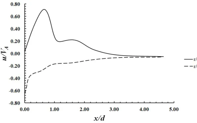
5.2.3 Longitudinal Variation of the Axial Velocity...81
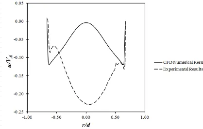
5.2.4 Radial Variation of Axial Velocity across the Shroud’s Diameter ...88
5.2.5 Axial Velocity Variation over Cycle at Certain Points of Interest in the Flow Field ...90
Chapter 6 CONCLUSIONS & RECOMMENDATIONS ...95
6.1 Conclusions ...95
6.1.1 Evaluation of the Simplified Numerical Model ...95
6.1.2 Comparison of Improved Numerical Model with Experiments ...95
6.2 Recommendations...96
Appendix A CAD DRAWINGS ... 98
A.1 Tank CAD Drawings ... 98
A.2 SJE CAD Drawings ... 100
A.3 Bench CAD Drawing ... 101
A.4 Scotch Yoke Mechanism CAD Drawings ... 102
Appendix B VERIFICATION OF SEEDING PARTICLE SIZE ... 106
Appendix C PIV SOFTWARE SET-UP ... 109
Appendix D PIV UNCERTAINTY MEASUREMENTS ... 112
D.1 Error in Calibration, 𝜶 ... 113
D.1.1 Image Length of the Calibration Target (Ruler) ... 113
D.1.2 Physical Length of the Calibration Target (Ruler) ... 113
D.1.3 Image Distortion ... 113
X
D.1.5 Ruler Position ... 114
D.1.6 Ruler Parallelism ... 114
D.2 Error in Displacement of the Particle Image, ∆𝒙 ... 114
D.2.1 Laser Power Fluctuations ... 114
D.2.2 Optical Distortion by CCD ... 114
D.2.3 Normal Viewing Angle ... 115
D.2.4 Mismatching Error... 115
D.2.5 Sub-Pixel Analysis ... 115
D.3 Error in the Time Interval, ∆𝒕 ... 115
D.3.1 Delay Generator ... 115
D.3.2 Pulse Timing Accuracy ... 115
D.4 Error in 𝜹𝒖 ... 116
D.4.1 Particle Trajectory ... 116
D.4.2 Three-Dimensional Effect ... 116
D.5 Dimensionless Axial Velocity Uncertainty (Uu/VA) ... 117
Appendix E NUMERICAL SOLUTION- FLUENT SET-UP ... 120
Appendix F TURBULENCE MODELLING LITERATURE REVIEW ... 126
F.1 k- 𝜺 Model ... 126
F.2 k-𝝎 Model ... 127
F.3 SST Model ... 128
Appendix G COMPLETE SET OF EXPERIMENTAL RESULTS .. 130
G.1 Period-Averaged Volume Flow Rate Exported from Fluent ... 130
G.2 Mean Flow Fields ... 132
G.3 Longitudinal Variation of the Axial Velocity ... 140
G.4 Radial Variation of Axial Velocity ... 148
REFERENCES ...152
XI
LIST OF TABLES
Table 3.1 General SJE Dimensionless Groups Optimum Operating Values ... 25
Table 3.2 The Optimized Dimensions & Parameters ... 27
Table 4.1 SJE Geometrical Parameters ... 46
Table 4.2 Under-Relaxation Factor for Each Variable ... 51
Table 4.3 The Error Percentage Difference between the 0.001 s and 0.0005 s Time Step Sizes for the Axial Velocity and the Period-Averaged Volume Flow Rate at the Specified Points ... 59
XII
LIST OF FIGURES
Figure 1.1 Synthetic Jet Formation ... 3
Figure 1.2 Schematic of SJE ... 4
Figure 2.1 Geometric Definitions of SJE and Conservation of Mass over a CV ... 11
Figure 2.2 Time-Averaged Centerline Velocity Versus Downstream Distance, where h is the Width of the Slot [12] ... 12
Figure 2.3 Parameters Governing the Synthetic Jet Ejector ... 14
Figure 3.1 Shroud- Actuator-Tank Arrangement with Dimensions ... 27
Figure 3.2 Schematic of the SJE CAD Model... 28
Figure 3.3 Isometric Drawing of the Piston and SJA ... 30
Figure 3.4 Components of the Scotch Yoke Mechanism ... 30
Figure 3.5 Experimental PIV Set-up ... 34
Figure 3.6 Calibration Image ... 35
Figure 3.7 The Circuit that Converts the Digital Signal from the Hall Sensor to a TTL Signal that Externally Triggers the Synchronizer ... 37
Figure 3.8 TTL Signals Generated by the Hall Sensor... 37
Figure 3.9 Captured Points within Dimensionless Time during a Cycle ... 38
Figure 4.1 Lin’s SJE Numerical Model Boundary Conditions [20] ... 44
Figure 4.2 Geometric Information for the SJE Solution Domain ... 46
Figure 4.3 SJE Numerical Model Boundary Conditions ... 49
XIII
Figure 4.5 Grid Refinement Convergence Study for Point A ... 54
Figure 4.6 Grid Refinement Convergence Study for Point B ... 54
Figure 4.7 The Selected Four Points to Determine the Axial Velocity Convergence within the Time Step Independence Study ... 56
Figure 4.8 Axial Velocity at One Diameter away from the Actuator’s Outlet along the Axis for Two Different Time Step Sizes ... 57
Figure 4.9 Axial Velocity at One Diameter away from the Actuator’s Outlet in the Middle Distance between the Shroud and the Actuator’s wall for Two Different Time Step Sizes ... 57
Figure 4.10 Axial Velocity at One and a Half Diameter away from the Actuator’s Outlet along the Axis for Two Different Time Step Sizes ... 58
Figure 4.11 Axial Velocity at One Diameter and a Half away from the Actuator’s Outlet in the Middle Distance between the Shroud and the Actuator’s wall for Two Different Time Step Sizes ... 58
Figure 5.1 A Phase-Averaged Volume Flow Rate Comparison between the Experimental Method, the Improved CFD Numerical Model and the Simplified Numerical Model at x/d=1.75 ... 62
Figure 5.2 Axial Velocity Variation across the Exit of the Orifice at t/T=0.2 ... 64
Figure 5.3 Axial Velocity Variation across the Exit of the Orifice at t/T=0.5 ... 64
Figure 5.4 Axial Velocity Variation across the Exit of the Orifice at t/T=0.8 ... 65
XIV
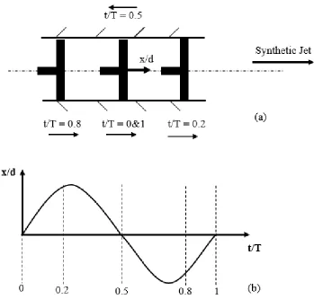
Figure 5.6 Specified Dimensionless Times within a Cycle a) Piston Position and Direction, b) Dimensionless Times ... 67
Figure 5.7 Velocity Field Vectors Obtained at t/T = 0.2 from (a) Phase-Averaging, 70
Figure 5.8 Velocity Field Vectors Obtained at t/T = 0.5 from (a) Phase-Averaging, 72
Figure 5.9 Velocity Field Vectors Obtained at t/T = 0.8 from (a) Phase-Averaging, 74
Figure 5.10 Instantaneous Flow Field at t/T=0.8 for Cycle a) 145 b) 1416 c) 1459 ... 79
Figure 5.11 The Variation of the Experimental Dimensionless Axial Velocity along the Flow Field Downstream at Three Locations at t/T = 0.2 ... 85
Figure 5.12 The Variation of the CFD Numerical Dimensionless Axial Velocity along the Flow Field Downstream at Three Locations at t/T = 0.2 ... 85
Figure 5.13 The Variation of the Experimental Dimensionless Axial Velocity along the Flow Field Downstream at Three Locations at t/T = 0.5 ... 86
Figure 5.14 The Variation of the CFD Numerical Dimensionless Axial Velocity along the Flow Field Downstream at Three Locations at t/T = 0.5 ... 86
Figure 5.15 The Variation of the Experimental Dimensionless Axial Velocity along the Flow Field Downstream at Three Locations at t/T = 0.8 ... 87
Figure 5.16 The Variation of the CFD Numerical Dimensionless Axial Velocity along the Flow Field Downstream at Three Locations at t/T = 0.8 ... 87
Figure 5.17 Velocity Profile across the Shroud’s Diameter at x/d = 1.75 for the Experiment and the Numerical Simulation at t/T = 0.2 ... 89
XV
Figure 5.19 Velocity Profile across the Shroud’s Diameter at x/d = 1.75 for the
Experiment and the Numerical Simulation at t/T = 0.8 ... 90
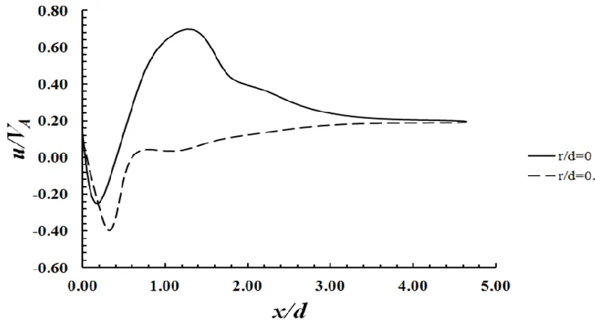
Figure 5.20 A Dimensionless Axial Velocity Comparison of the Experimental Method and the Improved CFD Numerical Model along the Axis at x/d = 1 ... 91
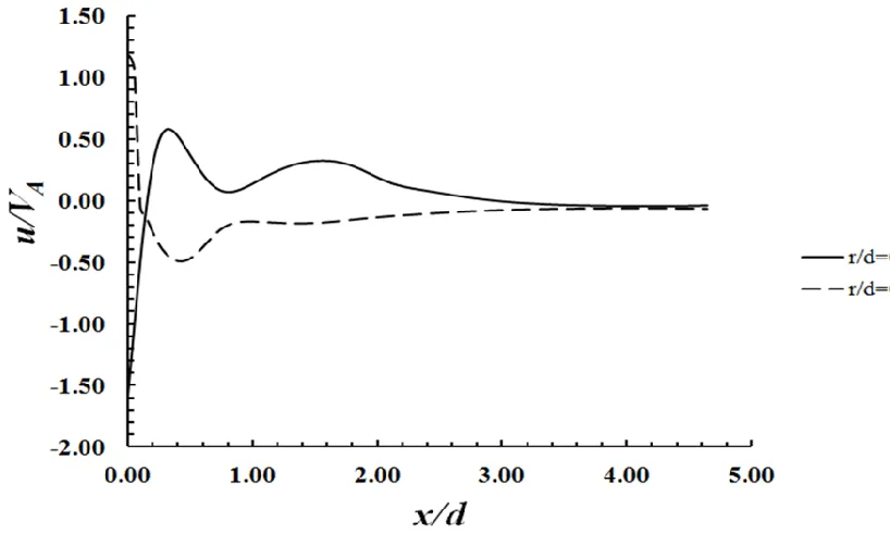
Figure 5.21 A Dimensionless Axial Velocity Comparison of the Experimental Method and the Improved CFD Numerical Model along the Axis at x/d = 1.5 ... 92
Figure 5.22 A Dimensionless Axial Velocity Comparison of the Experimental Method and the Improved CFD Numerical Model along the Centre of the Secondary Flow Inlet at x/d = 1 ... 93
Figure 5.23 A Dimensionless Axial Velocity Comparison of the Experimental Method and the Improved CFD Numerical Model along the Centre of the Secondary Flow Inlet at x/d = 1.5 ... 93
Figure A.1 Base of the Tank CAD Drawing ... 98
Figure A.2 The Smaller Side Walls CAD Drawing ... 99
Figure A.3 The Larger Side Walls CAD Drawing ... 99
Figure A.4 The Shroud, the Actuator and the Flange Integrated CAD Drawing . 100 Figure A.5 The Shroud Supports CAD Drawing (Acrylic Pieces and Threaded Rod) ... 100
Figure A.6 Bench CAD Drawing ... 101
XVI
Figure A.8 Yoke CAD Drawing ... 102
Figure A.9 Piston with Two O-rings CAD Drawings ... 103
Figure A.10 Rod (Connects between the Yoke and the Piston) CAD Drawing... 103
Figure A.11 Keyed Rotary Shaft CAD Drawing ... 104
Figure A.12 Square Key CAD Drawing ... 104
Figure A.13 Needle Bearing for the Yoke CAD Drawing ... 105
Figure A.14 Linear Bearing Drawing ... 105
Figure B.1 Dimensionless Time Versus Particle Velocity Results ... 108
Figure C.1 Component Setup Window from Insight 4G Software by TSI ... 109
Figure C.2 Capture Timing Setup Window from Insight 4G Software by TSI ... 111
Figure E.1 UDF Used to Move the Dynamic Mesh Periodically... 120
Figure G.1 Velocity Field Vectors Obtained at t/T= 0 from (a) Phase-Averaging, 133 Figure G.2 Velocity Field Vectors Obtained at t/T= 0.1 from (a) Phase-Averaging, ... 134
Figure G.3 Velocity Field Vectors Obtained at t/T= 0.3 from (a) Phase-Averaging, ... 135
Figure G.4 Velocity Field Vectors Obtained at t/T= 0.4 from (a) Phase-Averaging, ... 136
Figure G.5 Velocity Field Vectors Obtained at t/T= 0.6 from (a) Phase-Averaging, ... 137
XVII
Figure G.7 Velocity Field Vectors Obtained at t/T= 0.9 from (a) Phase-Averaging,
... 139
Figure G.8 The Change of the Experimental Dimensionless Axial Velocity Along the Flow Field Downstream at Three Locations at t/T=0 ... 141
Figure G.9 The Change of the CFD Numerical Dimensionless Axial Velocity Along the Flow Field Downstream at Three Locations at t/T=0 ... 141
Figure G.10 The Change of the Experimental Dimensionless Axial Velocity Along the Flow Field Downstream at Three Locations at t/T=0.1 ... 142
Figure G.11 The Change of the CFD Numerical Dimensionless Axial Velocity Along the Flow Field Downstream at Three Locations at t/T=0.1 ... 142
Figure G.12 The Change of the Experimental Dimensionless Axial Velocity Along the Flow Field Downstream at Three Locations at t/T=0.3 ... 143
Figure G.13 The Change of the CFD Numerical Dimensionless Axial Velocity Along the Flow Field Downstream at Three Locations at t/T=0.3 ... 143
Figure G.14 The Change of the Experimental Dimensionless Axial Velocity Along the Flow Field Downstream at Three Locations at t/T=0.4 ... 144
Figure G.15 The Change of the CFD Numerical Dimensionless Axial Velocity Along the Flow Field Downstream at Three Locations at t/T=0.4 ... 144
Figure G.16 The Change of the Experimental Dimensionless Axial Velocity Along the Flow Field Downstream at Three Locations at t/T=0.6 ... 145
XVIII
Figure G.18 The Change of the Experimental Dimensionless Axial Velocity Along the Flow Field Downstream at Three Locations at t/T=0.7 ... 146
Figure G.19 The Change of the CFD Numerical Dimensionless Axial Velocity Along the Flow Field Downstream at Three Locations at t/T=0.7 ... 146
Figure G.20 The Change of the Experimental Dimensionless Axial Velocity Along the Flow Field Downstream at Three Locations at t/T=0.9 ... 147
Figure G.21 The Change of the CFD Numerical Dimensionless Axial Velocity Along the Flow Field Downstream at Three Locations at t/T=0.9 ... 147
Figure G.22 Velocity Profile Across the Shroud’s Diameter at x/d=1.75 for the Experiment and the Numerical Simulation at t/T=0 ... 148
Figure G.23 Velocity Profile Across the Shroud’s Diameter at x/d=1.75 for the Experiment and the Numerical Simulation at t/T=0.1 ... 149
Figure G.24 Velocity Profile Across the Shroud’s Diameter at x/d=1.75 for the Experiment and the Numerical Simulation at t/T=0.3 ... 149
Figure G.25 Velocity Profile Across the Shroud’s Diameter at x/d=1.75 for the Experiment and the Numerical Simulation at t/T=0.4 ... 150
Figure G.26 Velocity Profile Across the Shroud’s Diameter at x/d=1.75 for the Experiment and the Numerical Simulation at t/T=0.6 ... 150
Figure G.27 Velocity Profile Across the Shroud’s Diameter at x/d=1.75 for the Experiment and the Numerical Simulation at t/T=0.7 ... 151
XIX
LIST OF ABBREVIATIONS/SYMBOLS
BC Boundary Condition
BDC Bottom Dead Centre
CAD Computer-Aided Design
CCD Charge-Coupled Device
CFD Computational Fluid Dynamics
CPU Central Processing Unit
CV Control Volume
DCC Direct Cross-Correlation
DFT Discrete Fourier Transform
DNS Direct Numerical Simulation
ECE Energy Cooling Efficiency
FBD Free Body Diagram
FEA Finite Element Analysis
FFT Fast Fourier Transform
FOV Field of View
IA Interrogation Area
ID Inner Diameter
ITTC International Towing Tank Conference LES Large Eddy Simulation
LDV Laser Doppler Velocimetry
Nd:YAG Neodym-Yttrium-Aluminum-Garnet
XX
PISO Splitting of Operators Scheme
PIV Particle Image Velocimetry
PIV-STD PIV Standardization
PTFE Polytetrafluoroethylene
QUICK Quadratic Upstream Interpolation for Convective Kinetics
RAM Random Access Memory
SJ Synthetic Jet
SJA Synthetic Jet Actuator
SJE Synthetic Jet Ejector
SST Shear Stress Transport
TDC Top Dead Centre
TSI Thermal System Inc.
TSPC Time Steps Per Cycle
TTL Transistor-Transistor Logic
UDF User Defined Function
VDC Volts Direct Current
VOF Volume of Fluid
VSJ Visualization Society of Japan
ZNMF Zero-Net Mass Flux
XXI
NOMENCLATURE
𝑎 Acceleration
𝐴 Surface Area of the Piston
𝐴𝑎 Amplitude Acceleration
𝐴𝑃 Primary Inlet Area
𝐴𝑆 Secondary Inlet Area
𝐵 Bias Error
𝐶𝑒 Entrainment Coefficient
𝑑 Synthetic Jet Orifice Diameter
𝐷 Synthetic Jet Actuator Diameter
𝐷𝐶 Direct Current
𝐷𝑒 Synthetic Jet Ejector Shroud Diameter
𝐷𝑇 Tank Diameter/Width
𝑓 Synthetic Jet Piston Driving Frequency
𝐹𝑃 Piston Force
𝐹𝑅 Bearing Force
𝑔 Gravitational Acceleration
𝐺 Gap between the OD of the Cavity and the ID of the Shroud
ℎ1 Height from the Orifice Exit to the Free Surface
𝐻 Height of Water in a Tank
𝑘 Integer between 1 and 𝑛
XXII
𝐿𝑒 Shroud Length
𝐿𝑜 Stroke Length
𝐿𝑜 𝑑
⁄ Dimensionless Stroke Length
𝐿𝐼𝐹 Laser-Induced Fluorescence
𝑚 Mass
𝑀𝑒 Entrained Mass Flow Rate Up to Position 𝑥
𝑀𝑗 Jet Mass Flow Rate at the Orifice
𝑀𝑆 𝑀𝑃
⁄ Pumping Effectiveness
∆𝑀𝑒 ∆𝑥
⁄ Entrainment Rate
𝑛 Number of Timesteps Per Cycle
𝑃 Pressure
∆𝑃 Pressure Difference
𝑄𝑖 Period-Averaged Inlet Volume Flow Rate
𝑄𝑜 Period-Averaged Outlet Volume Flow Rate
𝑄𝑃 Period-Averaged Primary Volume Flow Rate
𝑄𝑆 Period-Averaged Secondary Volume Flow Rate
𝑅 Synthetic Jet Orifice Radius
𝑅𝐴𝑁𝑆 Reynolds-Averaged Navier-Stokes
𝑅𝑒 Reynolds Number
𝑅𝑆 Synthetic Jet Ejector Shroud Radius
𝑅𝑇 Tank Radius
XXIII
𝑆 Stokes Number
𝑆𝑎 Amplitude Piston Displacement
𝑆𝑡 Strouhal Number
𝑡𝑡 Synthetic Jet Actuator Cavity Thickness
𝑡95% t Distribution Value at 95 % Confidence Level
𝑡 𝑇
⁄ Dimensionless Time
∆𝑡 Time Interval between Two Image Pairs in PIV Calculations
𝑇 Synthetic Jet Piston Driving Period
𝑇𝑇 Synthetic Jet Ejector Shroud Thickness
∆𝑇 Timestep Size
𝑈𝑟𝑚𝑠 RMS Axial Velocity
𝑈 Mean Velocity
𝑈̅ Time Integral Velocity over One Period
𝑈𝑜 Characteristic Velocity
𝑉𝐴 Velocity Amplitude
𝑉𝑝 Orifice Area-Average Velocity
𝜔 Angular Velocity
𝑊 Weight
𝑥 Axial Distance from the Orifice Exit Plane
XXIV
Greek Letters
𝜌 Water Density
𝜌𝑗 Water Jet Density at the Orifice
𝜌𝑠 Density of the Surrounding Atmosphere
𝜇 Water Dynamic Viscosity
𝜔 Turbulence Frequency
𝜗 Water Kinematic Viscosity
𝜎 Random Error
1
Chapter 1
INTRODUCTION
In fluid dynamics, a jet is defined as a stream of fluid that is projected through an
opening under pressure into a surrounding medium. Air that comes out of a hairdryer is
considered to be a submerged jet because the jet fluid is the same as the surrounding
medium. On the other hand, water that comes out of the garden hose to the surrounding
air is considered to be a non-submerged jet [1]. Jets that have an exit exposed to the
atmosphere are called free jets. Free jets may also be unsteady and not only used for mixing
but for other purposes, such as producing thrust. For unsteady jets, mean velocity and
pressure change with time, while they are constant with time for steady jets [2]. A special
case of unsteady jets is called a pulsating jet [3]. Pulsating jets have periodic pulsations
superimposed on the mean flow [4,5]. Constraining a jet by adding a shroud or a mixing
tube creates a confined jet [6]. The jet ejector is considered a special case of a confined jet
that can involve steady or pulsating jet. In this chapter, Synthetic Jets (SJs) and Synthetic
Jet Ejectors (SJEs) will be defined as well as the motivation and the scope of the thesis.
1.1Synthetic Jets (SJs)
A synthetic jet (SJ) is a special case of a pulsating jet with zero mean flow. They
are produced by the periodic vortices formed by alternating momentary ejection and
suction of fluid through an orifice on one side of a cavity whose volume is changed by
means of an oscillating mechanism [7]. An oscillating diaphragm or a piston can be used
2
[8] or using a piezoelectric wafer [9], and the jet flow is observed to become steady a short
distance downstream of the orifice exit.
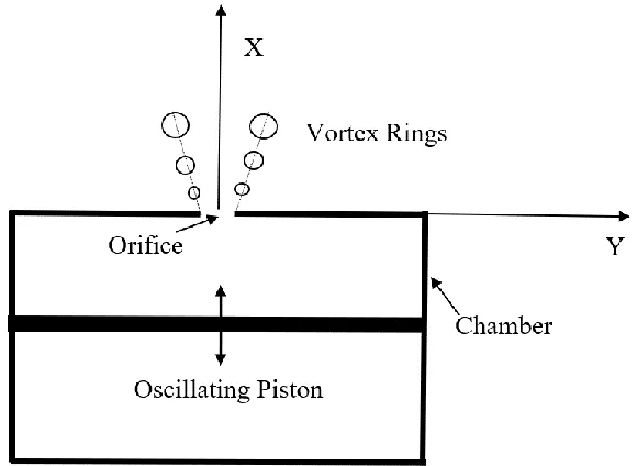
A Synthetic Jet Actuator (SJA) is a fluidic device that is used to produce synthetic
jets. The SJA includes three main parts: chamber or cavity, orifice and an oscillating driver
as shown in Figure 1.1. The movement of the oscillating driver causes the fluid to be
periodically entrained into and then expelled from the chamber through the orifice to the
atmosphere. Vortex rings can be generated around the orifice during the ejection phase of
the cycle, under certain operating conditions, as illustrated by Holman et al. [10], and travel
downstream from the orifice exit. The interaction of those vortex rings generates the SJ.
The self-induced velocity of the vortex ring and its distance away from the actuator’s
orifice control the degree of interaction between the vortex and the reversed flow through
the orifice, caused by the suction of the surrounding fluid [11]. Thus, the vortex ring will
die out during the suction phase if its self-induced velocity is not high enough to move it
away from the orifice exit. The jet flow becomes steady a short distance downstream of
3
Figure 1.1 Synthetic Jet Formation
1.1.1 Advantages of the Synthetic Jet
The main advantage of a synthetic jet is that it has a zero-net mass flux (ZNMF) at
the exit of the orifice. In other words, synthetic jets are formed completely from the
working fluid within the surroundings in which they are generated. Thus, it transfers linear
momentum to the surrounding flow without any external mass flow source or piping system
[4]. Smith and Swift [12] have also concluded that synthetic jets entrain more fluid than
continuous jets near the orifice exit due to their formation of vortices. Thus, the spread
and the volume flux of synthetic jets have a greater increase in the axial flow direction than
do continuous jets.
1.1.2 Synthetic Jet Applications
The advantages mentioned in the previous sub-section make synthetic jets a
desirable and an affordable choice in different applications. In the case of aerodynamics,
pressure-4
induced drag force by delaying the flow separation, as well as, shortening the length and
the thickness of the wake [11,12]. Also, synthetic jets can increase energy cooling
efficiency (ECE) by providing a high local heat transfer coefficient at a much lower flow
rate [8, 13, 15]. Moreover, synthetic jets can be used in thrust vectoring by deflecting the
mean flow of an engine jet from the centerline and manipulating the direction of thrust to
control the altitude and angular velocity of the vehicle [18].
1.2Synthetic Jet Ejector (SJE)
Simply, SJEs consist of two main parts: the shroud, or the mixing tube, and the
SJA, as shown in Figure 1.2. In the case of SJEs, the primary steady jet in a steady jet
ejector is replaced with a SJA, which creates a pressure difference between the fluid inside
the shroud and the fluid outside the shroud [19]. Thus, a secondary flow is entrained
through the gap between the actuator and the shroud as presented in Figure 1.2. Thereby,
the main goal of the shroud is to mix both flows and direct them to the other end of the
tube, where the total flow exits. Thus, SJEs can be thought of as a type of self-contained
fluidic pump.
5
1.3Motivation and Scope
The present thesis is a contribution to the ongoing SJE research here at the
University of Windsor. The experimental and numerical work included in this thesis is
used to evaluate the simplified numerical model reported in a previous M.A.Sc. thesis [20]
and used to estimate the optimum operating conditions.
The thesis is organized into six chapters. Chapter 2 starts with a discussion of
dimensionless SJE parameters, followed by synthetic jet characteristics, synthetic jet
parameters and a review of the literature that is pertinent to this study. Chapter 3 includes
a description of the SJE test facility, the PIV measurement facility, experimental procedure,
data reduction, and measurement uncertainty. The numerical model, boundary conditions,
grid, timestep determination, turbulence modelling, and solution methods are explained in
detail in Chapter 4. The results, including phase-averaged measurements and
period-averaged measurements, and the comparisons between the experimental data and the
simplified and the improved numerical models are presented in Chapter 5. Conclusions,
6
Chapter 2
LITERATURE REVIEW
This chapter begins by discussing general information including some of the
important dimensionless parameters previously used to characterize the flow of the
synthetic jets and synthetic jet ejectors. Synthetic jet parameters that control the flow
characteristics of synthetic jets formation are also discussed. The last section is devoted to
a discussion of some of the previous numerical and experimental studies that have been
reported in the literature regarding synthetic jets and synthetic jet ejectors.
2.1 Synthetic Jet Dimensionless Groups
The two most important dimensionless numbers that characterize the synthetic jet
flow fields are the Reynolds number and the Strouhal number. Defining a length, time and
velocity scale to be used in these numbers is necessary in order to non-dimensionalize the
flow field. The Reynolds number for a steady jet is defined as,
𝑅𝑒
𝑜=
𝑈
𝑜𝑑
𝜗
(2.1)where, 𝑈𝑜 is the characteristic velocity, 𝑑 is the orifice diameter and 𝜗 is the kinematic
viscosity. If the Reynolds number falls below 50, when the characteristic velocity is
defined using the amplitude jet exit velocity, the jet will not separate from the orifice edge,
7
suction phase [21]. The Strouhal number is based on oscillation frequency and the same
velocity scale and is shown in Equation 2.2,
𝑆𝑡
0=
𝑓𝑑
𝑈
𝑜 (2.2)A large Strouhal number means that the actuator cycles several times before fluid elements
pass through the orifice region, while, small a Strouhal number indicates that the fluid
elements pass through the orifice region in one cycle. The square root of the product of
Reynolds number and Strouhal number is known as the Stokes number, as given in
Equation 2.3. In this study, the Stokes number is the ratio between the thickness of the
unsteady boundary layer in the orifice (𝛿2 = 𝜗𝑓) to the orifice diameter. The orifice is not
strongly influenced by viscous effects if the Stokes number is large, while if the Stokes
number is small, the orifice is mostly controlled by viscosity, and the jet can choke on the
unsteady boundary layer [21].
𝑆 = √
𝑓 𝑑
2𝜗
(2.3)2.1.1 Characteristic Velocity, 𝐔𝐨
For steady jets, the time-mean of the area-averaged instantaneous velocity at the
orifice is selected to be characteristic velocity. A velocity scale is difficult to define for
synthetic jets since it is unsteady and periodic, as mentioned in Chapter 1. In this case, the
8
Many different methods have been used to define the characteristic velocity scale for the
SJ within the last twenty years. Kral et al. [22] considered the maximum value of the jet
instantaneous velocity as the characteristic velocity. Rizzetta et al. [23] used a
peak-to-peak orifice velocity value as the velocity scale. Mallinson et al. [24] took the averaged
velocity at some distance downstream from the orifice exit as the velocity scale. Utturkar
et al. [25] considered the spatial and time-averaged exit velocity during the ejection phase.
Smith & Glezer [9] only considered the mean-velocity over the ejection half of the period,
since the jet phenomenon is controlled by the ejection phase. Cater & Soria [26] proposed
a velocity scale that took into consideration the mean momentum flow.
Since this thesis is based on the evaluation of the optimum conditions from the
simplified model [20] for the SJE, the same velocity scale is used in this thesis. This is the
same velocity scale that was introduced by Smith & Glezer [9], and it defines the axial
velocity for only the ejection half cycle averaged over the cycle, as shown in Equation 2.4
𝑈
𝑜= 𝑓𝐿
𝑜=
1
𝑇
∫ 𝑉
𝑝(𝑡)𝑑𝑡
𝑇 2 ⁄ 0 (2.4)In Equation 2.4, 𝑓 is the piston oscillation frequency, T is the piston oscillating period,
𝑉𝑝(𝑡) is the orifice area-average velocity which is a function of time and 𝐿𝑜 is the stroke
length. The stroke length is defined as,
L
o= ∫ V
p(t)dt
T 2 ⁄
0
(2.5)
9
𝑉
𝑝= 𝑉
𝐴sin (2𝜋𝑓𝑡)
(2.6)Thus, the stroke length and the velocity scale can be simplified as follows,
𝐿
𝑜=
𝑉
𝐴𝜋𝑓
(2.7)
𝑈
𝑜=
𝑉
𝐴𝜋
(2.8)
2.1.2 Time-Averaged Quantities
For periodic flows, the time-averaged quantities are determined based on the net
effect over a full cycle. For example, the period averaged velocity, 𝑈̅, is defined as the
time integral of the velocity value over one period, T, divided by the period, as follows,
𝑈̅ =
1
𝑇
∫
𝑉(𝑡)𝑑𝑡
𝑇+𝑡
𝑡
(2.9)
where time is denoted by t, and V is the area-averaged time-dependant flow velocity.
The number of time steps per cycle (TSPC) is denoted by n,
𝑛 =
𝑇
∆𝑇
(2.10)
where ∆𝑇 is the timestep size. Thus, using the rectangular integration (Midpoint rule),
10
𝑈̅ =
∑
𝑉
𝑘𝑛 𝑘=1
𝑛
(2.11)
where k is an integer having values 1 to n inclusive [20].
As mentioned in Chapter 1, the SJE shroud involves three different flows: the
primary flow, which is generated by the actuator, the secondary flow, which is entrained
into the shroud, and the outlet flow, which is a mixture of the primary and secondary flows
that is directed out of the shroud. The time average of the primary volume flow rate over
one period, period-averaged, is equal to zero because of continuity and the fact that the
flow is incompressible. Thus, the period-averaged total volume flow rate equals to the
period-averaged secondary volume flow rate. The period area-averaged velocity is used to
calculate the period-averaged volume flow rate as shown in Equations 2.12, 2.13, 2.14 and
2.15. In Figure 2.1, the geometry of a simple axis-symmetric synthetic jet ejector is
presented. The orifice diameter is defined by d, the actuator diameter by D, the shroud
diameter by De and the shroud length by Le. Changing any of the above-mentioned
dimensions can cause a change in the flow. The symmetry line is parallel to the x-axis.
The center point of the orifice exit is considered to be the reference point in this study.
𝑄
𝑝𝑟𝑖𝑚𝑎𝑟𝑦= 𝑄
𝑃= 𝑈
̅̅̅̅ ∗ 𝐴
𝑃 𝑃= 0
(2.12)𝑄
𝑠𝑒𝑐𝑜𝑛𝑑𝑎𝑟𝑦= 𝑄
𝑠= 𝑈
̅̅̅ ∗ 𝐴
𝑠 𝑠 (2.13)11
𝑄
𝑜𝑢𝑡𝑙𝑒𝑡= 𝑄
𝑜= 𝑄
𝑠 (2.15)Generally, when the time-averaged flow rate becomes independent of the number
of cycles, the flow is considered to have reached a time-periodic steady state. For the
present numerical study, the criterion for this condition is taken to be when the secondary
inlet volume flow rate between two consecutive cycles is less than 0.5 %.
Figure 2.1 Geometric Definitions of SJE and Conservation of Mass over a CV
2.2 Synthetic Jet Ejector Characteristics
Synthetic Jets are created due to the periodic suction and ejection of fluid, by an
oscillating driver, through an orifice. Due to boundary separation, the fluid that is pushed
through the orifice rolls up and forms vortex rings during the ejection phase of the cycle.
During the suction phase, the ambient fluid near the jet exit gets drawn back through the
orifice into the actuator, as the expelled vortex ring travels away from the orifice due to its
12
cause the formed vortex ring to be sucked back into the actuator during the suction phase,
thus, preventing the formation of a SJ downstream Synthetic jets generate a high turbulence
level because of vortex pairs breakdown, due to its circumferential instability, which raises
the fluctuation level compared to other jets [29]. Generally, the flow field of the synthetic
jets can be classified into two regions: developing region and developed region. The
developing region occurs near the orifice exit, where the flow is mostly dominated by the
vortex rings. The developed region, which occurs at a distance away from the orifice exit
depending upon the jet exit geometry and the turbulence caused by the collapsed vortex
rings has the same characteristics as steady jets [30]. Thus, the time-averaged centerline
velocity of synthetic jets starts with a value of zero at the orifice exit and rises to a high
level at some distance downstream, before it starts decaying [12] according to the -1
power-law decay typical of circular jets [26] and the -1/2 power power-law for planar jets, as shown in
Figure 2.2.
13
2.2.1 Entrainment
Entrainment is the ability of a moving fluid to draw in additional fluid from the
surrounding fluid. It is one of the main characteristics for jets (both steady and synthetic)
and is the operational mechanism responsible in jet ejectors. The jet entrainment rate is
defined by the gradient of the entrained mass flow rate in the direction of jet flow, ∆𝑀𝑒/
∆𝑥, as first introduced by Ricou and Spalding [31] for a fully developed steady turbulent
axisymmetric jet. Hill [32] used Ricou and Spalding’s work to directly measure the local
entrainment rate in the initial region of an axisymmetric turbulent air jet to determine an
entrainment coefficient. The entrainment coefficient, which pertains to the ejector’s
performance, is provided by Vermeulen et al. [33] and summarized as follows,
𝐶
𝑒=
𝑑
𝑀
𝑗√
𝜌
𝑗𝜌
𝑠∆𝑀
𝑒∆𝑥
(2.16)Where 𝐶𝑒= entrainment coefficient
𝑀𝑗= jet mass flow rate at the orifice 𝜌𝑗= jet density at the orifice
𝜌𝑠= density of the surrounding atmosphere 𝑀𝑒= entrained mass flow rate up to position x
𝑥 = axial distance from the orifice exit plane
It was concluded by Smith and Swift [12] that synthetic jets entrain more fluid than
steady jets do due to the vortex rings formed. For the pulsating jet, it was observed that
the entrainment coefficient increased non-linearly with axial distance downstream of the
14
entrainment coefficient by up to 4.5 times greater than the non-driven case at x/d = 10, and
by up to 5.2 times at x/d = 17.5. Since 𝑀𝑗 is zero for synthetic jets and 𝑀𝑒 reaches a
constant value when the flow reaches a steady state, it is impossible to apply the
entrainment coefficient definitions.
In case of synthetic jets ejectors, the fluid is entrained into the primary flow inside
the shroud through the secondary inlets. The amount of the entrainment fluid through the
secondary inlets depends on the strength of the primary flow generated from the actuator
and the size of the secondary flow inlet area.
2.3 Synthetic Jet Ejector Parameters
There are many parameters that control the generation of synthetic jets and their
characteristics. The dimensionless groups that were discussed in Section 2.1 are obtained
from these parameters. Murugan et al. [29] divided the synthetic jet governing parameters
into three categories: actuator operating parameters, geometrical parameters, and fluid
parameters. The parameters are summarized in Figure 2.3.
15
2.4 Related Studies
A considerable number of studies have been conducted on the numerical and
experimental aspects of synthetic jets. On the other hand, not many studies have been
completed for synthetic jet ejectors. This section is divided into four subsections to review
the pertinent studies on synthetic jets, synthetic jet ejectors and the behavior of vortex rings
formed using a moving piston.
2.4.1 Synthetic Jets
Rayleigh [34,35] was first to notice that vibratory motion of a surface not only
generates sound but also causes many phenomena, including a regular air current which is
now called acoustic streaming. Eckart [36] developed a second-order mathematical model
accounting for the friction, that was the main cause of Rayleigh’s phenomena. This
mathematical model helped in calculating the steady flow produced by a sound beam of
circular cross-section. Subsequently, Ingard & Labate [37] used smoke to visualize the
fluid particles and to analyze the acoustical streaming phenomena around an orifice. A
sinusoidal motion was developed using acoustic waves and the smoke particle motion
visualized using stroboscopic illumination. Therefore, Ingard & Labate were the first to
observe what is not called a synthetic jet. In 1994, the first synthetic jet actuator was
introduced by Coe et al. [38].
2.4.1.1 Experimental Studies
James et al. [39] experimentally investigated a round turbulent submerged water jet
produced by a resonantly driven diaphragm mounted flush with a wall. Due to cavitation
bubbles formed on the diaphragm surface and the jet formation was hindered by the suction
16
jet. Smith & Glezer [9] evaluated the previous results by comparing the properties for a
two-dimensional synthetic jet to a two-dimensional steady jet, for Reynolds numbers that
ranged from 104 to 489 and Strouhal numbers from 0.04 to 0.19. They observed that the
width and the velocity of the flow produced by a synthetic jet were lower than that
generated by a steady jet. However, Cater & Soria [26] experimentally investigated a
round Zero Net Mass Flux (ZNMF) jet, for Reynolds numbers ranging from 1,000 to
10,000 and Strouhal numbers ranging from 0.0015 to 0.0072. They observed that in the
far field flow, the ZNMF has a cross-stream velocity distribution similar to that of a
conventional steady jet, but with a larger spreading rate. Eventually, Glezer & Amitay [4]
and Smith & Swift [12] observed that synthetic jets, with Re = 2,000 and St = 0.06, are
mainly controlled by vortex pairs near the orifice, which entrain more fluid than steady
jets. Thus, the width and the velocity of the synthetic jet are greater compared to the steady
jet.
Shuster & Smith [40] studied the flow properties of a round synthetic jet
experimentally, using PIV, with Reynolds numbers that ranged from 1,000 to 10,000 and
Strouhal numbers from 0.33 to 1. They found that round synthetic jets scales such as time
and length scales are defined using the dimensionless stroke length, 𝐿𝑜/𝑑. If the distance
from the orifice is less than 𝐿𝑜, the flow is completely dominated by vortex pairs during
the ejection phase, beyond which the flow is similar to a turbulent steady jet.
Agrawal & Verma [41] conducted a similarity analysis that was supported by
experimental data between a synthetic jet and a continuous jet flow field. It was concluded
17 2.4.1.2 Numerical Studies
Kral et al. [22] conducted two-dimensional incompressible numerical simulations
of a synthetic jet with a quiescent external flow. The actuator was prescribed as a
sinusoidal velocity profile using the velocity inlet boundary condition. This was done with
laminar and turbulent jets, but the laminar case was not able to capture the vortices
collapsing that were observed experimentally. Although the synthetic jet actuator operated
with ZNMF at the nozzle exit, the jet produced non-zero mean streamwise velocity.
A numerical study by Rizzetta et al. [23] was performed to investigate the interior
actuator cavity flow and external jet flow field using the unsteady compressible Navier-
Stokes equations and Direct Numerical Simulation (DNS). An oscillatory displacement
boundary condition was specified at the lower end of the cavity. It was shown that the
internal cavity flow becomes periodic after several cycles. Thus, only the external flow
domain was considered in their following simulations using a periodic velocity inlet
boundary condition at the actuator outlet. Also, it was noticed that the vortex breakdown
due to the spanwise instabilities was not captured using the 2-D simulations, so 3-D
simulations were conducted to overcome this issue.
Mallinson et al. [24] studied the synthetic jet flow both experimentally using a
single hot-wire anemometer, and computationally, using the commercial software package
CFX4.2. The experimental and the computational results for the velocity profile
distribution were found to be very similar although the results near the exit were
questionable due to the directional ambiguity of the hot-wire. It was discovered that the
inertia (diaphragm forcing) and viscous (orifice boundary layer) forces are the main factors
18
Rampunggoon [28] numerically investigated the dynamics of synthetic jets in the
presence of cross-flow as well as jets issuing into quiescent air using an incompressible
Navier-Stokes solver in a two-dimensional configuration. A thorough parametric study of
the jet characteristics was conducted by changing various parameters. The diaphragm
amplitude, external flow Reynolds number, boundary layer thickness, and slot dimensions
were all varied to observe the resulted changes on the flow. It was noticed that large mean
recirculation bubbles are formed in the external boundary layer only if the jet velocity is
significantly higher than the cross-flow velocity.
Kral et al. [22], Lee & Goldstein [42] again used the DNS method to study the
effects of fluid and geometric parameters on the resulting flow field in two-dimensional
slot synthetic jets pulsing into an initially quiescent flow. A more uniform velocity profile
at the orifice and an increase in the vortex formation rate can be achieved by a thicker
orifice lip. Compared with the round orifice lip, a straight orifice lip changed the orifice
velocity profile, but the synthetic jet flow field and the formation of vortices were not
affected.
Utturkar et al. [25,43] conducted two-dimensional numerical simulations to
indicate how the design of the jet cavity would affect synthetic jets by taking into
consideration the placement of the oscillating diaphragm and the changes in the cavity
aspect ratio. Also, the authors evaluated a jet formation criterion, which was based on
𝑅𝑒𝑈𝑜
𝑆2 , for two-dimensional and axisymmetric synthetic jets. Furthermore, the authors have concluded the use of an axisymmetric orifice as the recommended method for generating
19
Fugal [44] also used Reynolds-averaged Navier-Stokes (RANS) to study how the
synthetic jet characteristics would be affected by changing the orifice exit geometry and
the dimensionless stroke length. It was observed that the k-𝜀 turbulence model more
accurately predicts the downstream behavior of the jet than the other RANS turbulence
models. It was also concluded that increasing the exit radius increases the magnitude of
the stroke length required to generate a jet.
Ravi et al. [45] conducted a three-dimensional numerical simulation to study how
synthetic jets with a larger aspect ratio develop when they are introduced into quiescent
air. They used a finite difference based Cartesian grid immersed boundary solver, which
is capable of simulating flows with complex 3-D, stationary and moving boundaries. It
was found that the vortex train originating from the orifice exit undergoes axis-switching
and assumes a complex shape. It was concluded, based on the mean shape of the flow field
and the jet spreading, that synthetic jets enhance entrainment of the surrounding fluid.
Jagannatha et al. [46] numerically developed a two-dimensional time-dependent
synthetic jet model. The authors stated that the most accurate simulation of the synthetic
jet must be accomplished with a 3-D model in order to fully capture the flow behavior.
However, the authors added that the synthetic jet behavior can be sufficiently described by
a 2-D model that includes a moving piston or a vibrating membrane. They
dynamic-layering technique that is simulated by a User Defined Function (UDF) from the Fluent
solver was used to represent the piston movement in this simulation. Also, the selection of
a proper turbulence model is required since the oscillating nature of the flow could result
in some intensely localized fluctuations. It was determined that k- 𝜔 SST is the best
20
concluded that the simulation was able to capture the synthetic jet vortices, the flow field,
and heat transfer characteristics related to the pulsating jet cooling.
2.4.2 Vortex Ring Generation Using a Moving Piston
In 1979, Didden [47] investigated the separated flow and the vortex circulation
from the flow produced by ejecting fluid from a circular nozzle by means of an
impulsively-started piston. The experiment was conducted using Laser-Doppler
Velocimetry (LDV) technique. It was concluded that the circulation generated from this
experiment, using a piston, underestimates the strength of the ring by approximately 25 %
compared to the models where constant velocity profiles across the nozzle’s cross section
was assumed.
Allen and Auvity [48] used Didden’s [47] geometry and circulation model to study
the effect of the piston vortex, which is formed in front of the advancing piston within the
cylinder, on the primary vortex ring that is generated at the orifice exit. The experiment
was carried out by a moving piston ejecting fluid from a tube into a large tank. It was
concluded that a piston finishing flush with the exit plane produces vortex rings with
significant flow complexity. The piston vortex is injected and entrained into the primary
vortex which resulted in an added impulse to the vortex ring. They also found evidence of
a centrifugal instability on the piston vortex which generates vortex filaments in a plane
perpendicular to the azimuthal direction. Also, some vorticity filaments, due to the
centrifugal instability on the piston vortex, were detected in the plane perpendicular to the
azimuthal direction. They found that the piston vortex reduces the distance that the ring is
21
2.4.3 Synthetic Jet Ejector
Vermeulen et al. [49] conducted both numerical and experimental studies to show
that adding a pulsation to a steady primary jet flow improves the ejector’s performance.
They also considered the special case of synthetic jet and showed that a “strong” synthetic
jet actuator that is pulsed at 131 Hz with a velocity of 91 m/s for the zero primary jet
velocity gives ejector performance as good as a pulsed high-velocity flow jet using a 150
W loudspeaker. The pumping effectiveness, defined as the mass flow rate ratio of
secondary to primary flows, 𝑀𝑠
𝑀𝑃 , increased by up to 4.5 times that for a steady jet. It is speculated that the pumping effectiveness improvement was due to the high velocity at the
boundary of the jet which is caused by the vortices generated. It was also observed that
the majority of the entrainment happens at the initial vortex immediately downstream of
the orifice exit. It was concluded by Meng [50] that SJEs enhance the entrainment better
than the pulsating jets and rotor valve pumps. For long experiments, controlling the
chamber’s temperature was considered the only disadvantage of the SJE for that conducted
experiment.
Lin [20,51] numerically investigated the behavior of particular configuration of
synthetic jet ejector. An efficient numerical model was developed, and an extensive
parametric study conducted. Univariate search optimization method was applied to
determine the set of parameters that yield the maximum flow rate. Thus, optimum SJE
dimensionless groups were then generated and summarized. This optimum configuration
was then investigated for the use in an innovative seat ventilation system. For the
simplified numerical model developed, the velocity profile is uniform across the primary
22
assumed that the secondary flow inlet has a constant pressure profile with a zero-gauge
pressure that was implemented as a pressure inlet condition. The shroud exit was set to
atmospheric pressure and implemented as a pressure outlet condition. The final grid used
after conducting a grid convergence study contains 400 × 120 cells. The final timestep
size, after conducting a timestep convergence study, was 1.38 × 10⁻⁵ s. The turbulence
model used for this study was 𝑘 − 𝜀.
2.4.3.1 SJE Applications
Mahalingam & Glezer [52] designed and built a synthetic jet ejector that operated
as an air-cooled heat sink. This module consists of a plate-fin heat sink integrated with
synthetic jet actuators. The synthetic jet module contains a plenum that is driven by
electromagnetic actuators. Each fin of a plate-fin heat sink is straddled by a pair of
synthetic jets. Thus, the ejector system trails the cool air upstream of the heat sink and
discharges it into the channels. It was concluded that the heat transfer coefficient generated
using synthetic jet ejectors are 150 % greater than those generated using steady jets.
Mahalingam & Glezer [53] studied how synthetic jet ejectors can be used to
augment the cooling provided by a global fan flow by reducing flow bypass. Flow bypass
is defined that it is the air flowing above and around heat sinks that results in significant
reduction in the amount of flow entering a heat sink. Adding synthetic jets upstream of the
inlet to the heat sink allows re-entrainment of the inlet flow to reduce flow bypass. It was
stated that synthetic jets helped to augment the heat dissipation of a heat sink by 25-35 %.
Later, Mahalingam et al. [54] added that doubling the jet speed led to a 20 % increase in
23
reducing the noise level by 9 dBA, as it allowed the dual fans to operate at 6500 RPM
instead of 9000 RPM.
2.4.4 Summary
It is shown from the literature that not many studies have been completed of
synthetic jet ejectors. Also, none of the studies found regarding SJEs include a combined
numerical and experimental studies. For instance, the simplified numerical solution [20]
lacked an experimental validation. Furthermore, previous studies can be found regarding
submerged SJs in water [8–10, 55, 56], but no studies known to the author exists on
analyzing SJEs with water as a working fluid. Thus, this thesis focuses on the behaviour
of SJEs in water, both experimentally and numerically.
2.5Objectives
The main goal of this research is to evaluate the accuracy of the 2-D SJE model
developed by Lin to determine the optimum conditions [20]. For this purpose, the flow
field of the SJE with optimum geometry and operating conditions is investigated in detail
using PIV experiments and numerical simulations. The specific objectives are as follows:
To design and construct a SJE test facility with water as the working fluid that
is dynamically similar to the optimum conditions from the simplified model.
To measure the velocity fields using Particle Image Velocimetry (PIV) and
determine the period-averaged volume flow rate experimentally.
To develop a more realistic CFD model based on the optimum conditions from
24
To use the more realistic numerical model to evaluate the assumptions made in
the simplified numerical model and compare their predicted phase-averaged
volume flowrate variation throughout the cycle with the experimental results.
To compare the details of the experimental velocity results with the new,
25
Chapter 3
EXPERIMENTAL METHOD
This chapter begins by introducing the constraints, and the selected SJE geometry
for this study, which is based on the previously reported optimum SJE conditions [20].
Mechanical design of the SJE test facility are provided followed by the description of the
phase-averaged velocity measurements using PIV technique. The experimental procedure
and data reduction techniques are then explained in detail. The last section is devoted to
the discussion of the method that is used to estimate the PIV measurements uncertainty.
3.1 SJE Geometry Selection
The predicted optimum dimensionless parameters that yield the maximum flow rate
out of the synthetic jet ejector studied and presented in Lin’s thesis [20] are summarized in
Table 3.1
Table 3.1 General SJE Dimensionless Groups Optimum Operating Values
Dimensionless Group (Pi Terms) Optimum Value 𝑄𝑠
𝐷𝑒2𝑉𝐴 0.262
𝑑 𝐷𝑒 ⁄ 0.8 𝐷 𝐷𝑒 ⁄ 0.8 𝐿𝑒 𝐷𝑒 ⁄ 4 𝑓 𝐷𝑒
𝑉𝐴 0.323
𝜌 𝑉𝐴 𝐷𝑒
𝜇 20,000
∆𝑝
26
One requirement in the design of the experimental flow facility is that flow
visualization of dye traces and quantitative velocity measurement techniques such as laser
Doppler anemometry can easily be applied. All these techniques are more easily applied
in liquids hence, it was decided to use water as the working fluid. The arrangement of the
experimental facility is shown in Figure 3.1. The SJE axis is vertical with the actuator
fastened to the bottom of a larger tank containing water. The shroud is also fastened to the
tank bottom so that it is co-axial with the actuator. The shroud and tank walls are plexiglass
to allow flow visualization. The tank size was selected to be 1 m3 in volume, 1m × 1m ×
1m. Since the water in the tank containing the ejector must approximate a stationary media
and the fact that the water has a free surface, it is necessary to use a large tank. In order to
allow good spatial resolution for measurements and flow visualization within the shroud,
the inside diameter of the shroud, 𝐷𝑒, is selected to be equal to 10 cm, which resulted in an
outer diameter value of 10.7 cm, considering standard size tubes. Based on the shroud
diameter selection and the optimum conditions obtained from the simplified model, the
remainder of the SJE parameters are calculated and summarized in Table 3.2.
According to the optimized dimensions, as presented in Table 3.2, the actuator’s
diameter, D, is equal to the orifice diameter, d, which means that the actuator wall thickness
is zero which is impossible to implement in practice. Moreover, the highlighted flow rate,
from Table 3.2, corresponds to the periodic-averaged secondary volume flow rate, which
27
Table 3.2 The Optimized Dimensions & Parameters
Parameter Value
Tank width (m) 1.0000
Shroud Diameter (De) (m) 0.1070 Actuator Diameter (D) (m) 0.0805 Orifice Diameter (d) (m) 0.0805 Shroud Length (Le) (m) 0.4000 Amplitude Velocity (Va) (m/sec) 0.1873
Frequency (f)(Hz) 0.5654
Period (T) (s) 1.7687
Stroke Length (Lo) (m) 0.1054
Amplitude (Sa) (m) 0.0527
Secondary Flow Rate (Qs) (m3/sec) 0.00056 Angular Velocity (w) (rad/sec) 3.5525 Amplitude Acceleration (Aa) (m/s2) 0.6654 Shroud Average Velocity (m/sec) 0.0625 Return Average Velocity (m/sec) 0.0006
28
3.2 SJE Test Facility
This section describes the main components of the SJE test facility and its
specifications. Figure 3.2 shows a schematic CAD model for the SJE design, excluding
the tank walls. All components are positioned on the top of the bench that is made of
welded angle iron.
Figure 3.2 Schematic of the SJE CAD Model
3.2.1 The Containment Tank
As stated previously, the tank is filled with water, and the actuator and the shroud,
which are the main components of the SJE, are centered on the base of the tank as shown
in Figure 3.2.
The tank is made of five clear optical acrylic sheets, one for the base and one for