University of Windsor University of Windsor
Scholarship at UWindsor
Scholarship at UWindsor
Electronic Theses and Dissertations Theses, Dissertations, and Major Papers
2012
Extension of graph clustering algorithms based on SCAN method
Extension of graph clustering algorithms based on SCAN method
in order to target weighted graphs
in order to target weighted graphs
Anton Chertov University of Windsor
Follow this and additional works at: https://scholar.uwindsor.ca/etd
Recommended Citation Recommended Citation
Chertov, Anton, "Extension of graph clustering algorithms based on SCAN method in order to target weighted graphs" (2012). Electronic Theses and Dissertations. 5408.
https://scholar.uwindsor.ca/etd/5408
This online database contains the full-text of PhD dissertations and Masters’ theses of University of Windsor students from 1954 forward. These documents are made available for personal study and research purposes only, in accordance with the Canadian Copyright Act and the Creative Commons license—CC BY-NC-ND (Attribution, Non-Commercial, No Derivative Works). Under this license, works must always be attributed to the copyright holder (original author), cannot be used for any commercial purposes, and may not be altered. Any other use would require the permission of the copyright holder. Students may inquire about withdrawing their dissertation and/or thesis from this database. For additional inquiries, please contact the repository administrator via email
Extension of graph clustering algorithms based on SCAN method in order to target weighted graphs
by
Anton Chertov
A Thesis
Submitted to the Faculty of Graduate Studies through School of Computer Science in Partial Fulfillment of the Requirements for
the Degree of Master of Science at the University of Windsor
Windsor, Ontario, Canada
2012
Extension of graph clustering algorithms based on SCAN method in order to target weighted graphs
by
Anton Chertov
APPROVED BY:
______________________________________________ Dr. Myron Hlynka, External Examiner
Mathematics and Statistics Department
______________________________________________ Dr. Luis Rueda, Internal Reader
School of Computer Science
______________________________________________ Dr. Scott Goodwin, Co-Advisor
School of Computer Science
______________________________________________ Dr. Ziad Kobti, Co-Advisor
School of Computer Science
______________________________________________ Dr. Boubakeur Boufama, Chair of Defence
School of Computer Science
DECLARATION OF CO-AUTHORSHIP / PREVIOUS PUBLICATION
I. Co-Authorship Declaration
I hereby declare that this thesis incorporates material that is result of joint research, as
follows: this thesis incorporates the outcome of a joint research undertaken in
collaboration and under supervision of Dr. Ziad Kobti and Dr. Scott Goodwin. The
collaboration is covered in Chapter 2 of the thesis. In all cases, the key ideas, primary
contributions, experimental designs, data analysis and interpretation, were performed by
the author, and the contribution of co-authors was primarily through the provision of
guidance and supervision.
I am aware of the University of Windsor Senate Policy on Authorship and I
certify that I have properly acknowledged the contribution of other researchers to my
thesis, and have obtained written permission from each of the co-author(s) to include the
above material(s) in my thesis.
I certify that, with the above qualification, this thesis, and the research to which it
refers, is the product of my own work.
II. Declaration of Previous Publication
This thesis includes 1 original paper that have been previously published/submitted for
Thesis Chapter Publication title/full citation Publication status*
Chapter 2 Weighted scan for modeling cooperative
group role dynamics. In Computational
Intelligence and Games (CIG), 2010 IEEE
Symposium on, pages 17 –22, aug. 2010
published
I certify that I have obtained a written permission from the copyright owner(s) to
include the above published material(s) in my thesis. I certify that the above material
describes work completed during my registration as graduate student at the University of
Windsor.
I declare that, to the best of my knowledge, my thesis does not infringe upon
anyone’s copyright nor violate any proprietary rights and that any ideas, techniques,
quotations, or any other material from the work of other people included in my thesis,
published or otherwise, are fully acknowledged in accordance with the standard
referencing practices. Furthermore, to the extent that I have included copyrighted
material that surpasses the bounds of fair dealing within the meaning of the Canada
Copyright Act, I certify that I have obtained a written permission from the copyright
owner(s) to include such material(s) in my thesis.
I declare that this is a true copy of my thesis, including any final revisions, as
approved by my thesis committee and the Graduate Studies office, and that this thesis has
ABSTRACT
In this thesis we evaluate current neighbour-based graph clustering algorithms: SCAN,
DHSCAN, and AHSCAN. These algorithms possess the ability to identify special nodes
in graphs such as hubs and outliers. We propose and extension for each of these in order
to support weighted edges. We further implemented two graph generating frameworks to
create test cases. In addition we used a graph derived from the ENRON email log. We
also implemented a Fast Modularity clustering algorithm, which is considered as one of
the top graph clustering algorithms nowadays. One of three sets of experiments showed
that results produced by extended algorithms were better than one of the reference
algorithms, in other words more nodes were classified correctly. Other experiments
revealed some limitations of the newly proposed methods where we noted that they do
not perform as well on other types of graphs. Hence, the proposed algorithms perform
DEDICATION
I dedicate this work to my family: my parents Nina and Mikhail and my brother Andrew.
ACKNOWLEDGEMENTS
It is an honour to thank people who made this work possible.
Great thanks to my co-advisor Dr. Scott Goodwin, who made my acceptance to
University of Windsor possible and provided me with guidance in University of Windsor
and Canada in general.
My sincere thanks to my co-advisor Dr. Ziad Kobti for his endless energy and
guidance through my research work.
Deepest thanks to Graduate Secretary Mandy Turkalj for her patience in
answering my countless organizational questions.
Also I would like to thank the most important people who contributed to my
research: my family. Thanks to my brother Andrew I happened to be accepted to
University of Windsor. Thanks to my parents Nina and Mikhail I was able to see this
TABLE OF CONTENTS
DECLARATION OF CO-AUTHORSHIP / PREVIOUS PUBLICATION ... iii
ABSTRACT ...v
DEDICATION ... vi
ACKNOWLEDGEMENTS ... vii
LIST OF TABLES ...x
LIST OF FIGURES ... xi
CHAPTERS 1 I. INTRODUCTION 1 I.1. Existing clustering algorithms ...1
I.2. Current research motivation ...2
I.3. Thesis contribution ...3
I.4. Thesis outline ...5
II. REVIEW OF LITERATURE 6 II.1.Graph clustering ...6
II.1.1. SCAN ... 9
II.1.2. DHSCAN ... 14
II.1.3. AHSCAN ... 16
II.1.4. WEIGHTED GRAPHS ... 18
II.2.Quality measurements ...20
II.2.1. NEWMAN'S MODULARITY ... 21
II.2.2. NOVEL SIMILARITY-BASED MODULARITY ... 22
II.2.3. PERFORMANCE ... 23
II.3.Graph Generators ...24
II.3.1. PLANTED L-PARTITION MODEL ... 24
II.3.2. PREFERENTIAL ATTACHMENT ... 26
II.3.4. COMMUNITY STRUCTURE ... 28
III. DESIGN AND METHODOLOGY 30 III.1. Extended structural similarity ...30
III.2. Clustering quality assessment ...33
III.2.1. NEWMAN'S MODULARITY ... 33
III.2.2. SIMILARITY-BASED MODULARITY ... 34
III.2.3. PERFORMANCE ... 38
III.3. Graph generators ...39
III.3.1. PLANTED L-PARTITION MODEL ... 39
III.3.2. OTHER TYPES OF GRAPHS ... 40
III.4. Complexity analysis ...41
III.5. Approach ...41
IV. ANALYSIS OF RESULTS 42 IV.1. Generated (random) graphs ...42
IV.1.1. PLANTED L-PARTITION MODEL ... 42
IV.1.1.1. DHSCAN AND AHSCAN ...42
IV.1.1.2. OVERALL PICTURE ...44
IV.1.2. POWER LAWS AND PREFERENTIAL ATTACHMENT ... 62
IV.1.3. REAL DATASET (ENRON) ... 67
V. CONCLUSIONS AND FUTURE WORK 70 REFERENCES ...73
LIST OF TABLES
TABLE 1-WEIGHTED AND UNWEIGHTED STRUCTURAL SIMILARITY-BASED MODULARITY. 36
TABLE 2-WEIGHTED AND UNWEIGHTED SIMILARITY-BASED MODULARITY VALUES ... 37
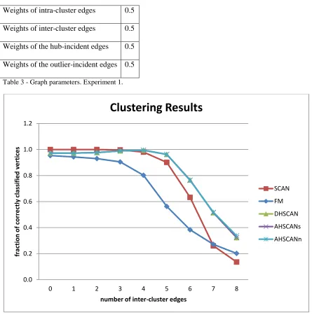
TABLE 3-GRAPH PARAMETERS.EXPERIMENT 1. ... 45
TABLE 4-STANDARD DEVIATION VALUES ... 46
TABLE 5-GRAPH PARAMETERS.EXPERIMENT 2. ... 51
TABLE 6-GRAPH PARAMETERS.EXPERIMENT 3. ... 52
TABLE 7-WEIGHT DISTRIBUTION.EXPERIMENT 4 ... 53
TABLE 8-WEIGHT DISTRIBUTION.EXPERIMENT 5 ... 55
TABLE 9-FINAL EXPERIMENT.WEIGHTS DISTRIBUTION.MAXIMUM INTRA/INTER RATIO. 57 TABLE 10-STANDARD DEVIATION VALUES ... 63
LIST OF FIGURES
FIGURE 1-SCAN PSEUDOCODE ... 13
FIGURE 2-DHSCAN PSEUDOCODE ... 16
FIGURE 3-AHSCAN PSEUDOCODE ... 18
FIGURE 4-COMMUNITY STRUCTURE WITH 1 INTER-CLUSTER EDGE PER NODE ... 25
FIGURE 5-COMMUNITY STRUCTURE WITH 4 INTER-CLUSTER EDGES PER NODE ... 26
FIGURE 6-COMMUNITY STRUCTURE WITH 6 INTER-CLUSTER EDGES PER NODE ... 26
FIGURE 7-CLUSTERING COEFFICIENT ... 29
FIGURE 8- STRUCTURAL SIMILARITY. ... 31
FIGURE 9-SAMPLE GRAPH WITH PLAIN WEIGHT DISTRIBUTION ... 35
FIGURE 10-GRAPH WITH DIFFERENT WEIGHT DISTRIBUTION ... 37
FIGURE 11-SYNTHETIC GRAPH WITH HUBS AND OUTLIERS ... 40
FIGURE 12-REGULAR (UNWEIGHTED)DHSCAN DETECTING SPECIAL NODES. ... 43
FIGURE 13-FRACTION OF VERTICES CLASSIFIED CORRECTLY.. ... 45
FIGURE 14-DETECTION OF SPECIAL NODES BY VARIOUS ALGORITHMS. ... 47
FIGURE 15-DIFFERENT QUALITY MEASUREMENTS OF DHSCAN CLUSTERING RESULTS.. 48
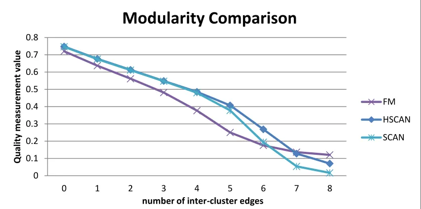
FIGURE 16-MODULARITY VALUES ... 49
FIGURE 17-SIMILARITY-BASED MODULARITY VALUES ... 50
FIGURE 18-PERFORMANCE VALUES. ... 50
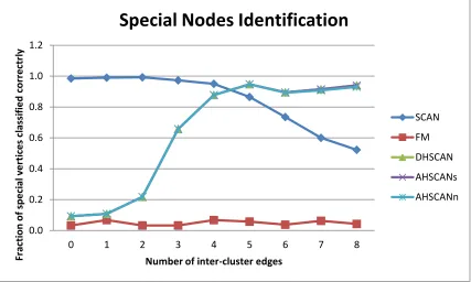
FIGURE 19-FRACTION OF SPECIAL NODES CLASSIFIED CORRECTLY.. ... 51
FIGURE 20-FRACTION OF VERTICES CLASSIFIED CORRECTLY. ... 52
FIGURE 22-FRACTION OF SPECIAL NODES IDENTIFIED CORRECTLY. ... 55
FIGURE 23-STRENGTHENING OF COMMUNITY STRUCTRUE YIELDS BETTER PARTITIONS ... 56
FIGURE 24-GRAPH CLUSTERING QUALITY MEASUREMENTS... 57
FIGURE 25-THE RATIO OF CORRECTLY CLASSIFIED VERTICES ... 58
FIGURE 26-QUALITY MEASUREMENTS OF DHSCAN PRODUCED PARTITIONS.. ... 59
FIGURE 27-MODULARITY VALUES FOR DIFFERENT PARTITIONS ... 60
FIGURE 28-SIMILARITY-BASED MODULARITY FOR DIFFERENT PARTITIONS. ... 60
FIGURE 29-PERFORMANCE VALUES FOR DIFFERENT PARTITIONS. ... 61
FIGURE 30-QUALITY MEASUREMENTS FOR RANDOM GRAPHS WITH 50 VERTICES. ... 63
FIGURE 31-QUALITY MEASUREMENTS FOR RANDOM GRAPHS WITH 100 VERTICES.. ... 64
FIGURE 32-QUALITY MEASUREMENTS FOR RANDOM GRAPHS WITH 200 VERTICES ... 65
FIGURE 33-A TYPICAL GRAPH WITH 200 NODES AND 400 EDGES FM CLUSTERING ... 66
FIGURE 34-SAME GRAPH CLUSTERED BY DHSCAN.. ... 66
FIGURE 35-FAST MODULARITY CLUSTERING OF ENRON DATASET ... 68
FIGURE 36-AHSCAN CLUSTERING OF ENRON DATASET ... 68
CHAPTER I
INTRODUCTION
A graph, or network, is a structure formed by a set of vertices (or nodes) and set of edges
connecting the vertices. This mathematical abstraction can be used to model various
real-world structures of interest to modern scientific applications. Graph clustering, or
partitioning, involves identifying groups of vertices in a graph that are tightly connected
to each other within a group, or has a high level of similarity of some kind, and are
weakly connected to vertices from other groups or are dissimilar to them. Further we will
use the words 'graph' and 'network', 'clustering and 'partitioning', 'node' and 'vertex',
'cluster' and 'community' interchangeably. Graph clustering has a great importance in
almost any field of modern science including biology, geology, geography, computer
science, engineering and social sciences. The latter is of specific interest to us. In social
networks, clustering enables the modeling and identification of hidden structures
(communities) that might not be seen to the observer or even to their members.
I.1.Existing graph clustering algorithms
Great amount of graph clustering algorithms exist today and one can find a lot of
information about them in survey on graph clustering by Schaeffer [10]. The deeper
insight of the graph clustering and related problems is given by Santo and Fortunato in
[28]. Graph clustering is a very vast topic, but in many cases the central idea behind it is
defining the similarity function between vertices of the graph. The further grouping of
vertices into communities is based on the value of this function, which defines whether
analysis, the notion of vertex neighbourhood seems very important to us. Intuitively
people sharing many friends are very likely to know each other and thus to be connected.
For that reason we would like to pay attention to algorithms that use adjacent vertices as
information for similarity functions: SCAN (Structural Clustering Algorithm for
Networks) [35] and two more algorithms derived from it: DHSCAN (Divisive
Hierarchical Structural Algorithm for Networks) [36] and AHSCAN (Agglomerative
Hierarchical Structural Algorithm for Networks) [37]. Designed by the same group of
scholars, these algorithms are based on structural similarity function which utilizes
information about vertex neighbourhood structure. Some of the mentioned algorithms are
also peculiar for their ability to detect vertices that play special roles in graphs: hubs
(connect different clusters, but don't belong to any certain one) and outliers (isolated
vertices). In social network analysis (especially in epidemiology, marketing, etc.) this
knowledge may be crucial.
I.2.Current research motivation
The initial form of SCAN and derived algorithms target only unweighted graphs, which
we identify as a serious limitation to their application. For instance, distance between
individuals (or degree of their attraction to each other) may be represented by a weight of
the edge connecting them. The further the individuals are located from each other, the
larger is the weight, the weaker is their ability to communicate (or as the attraction
increases, the interaction becomes easier). In [4] a weighted version of SCAN which
allows it to overcome the mentioned limitations was introduced. However, the new
algorithm. Moreover, the formula for structural similarity used for Weighted SCAN at the
same time introduces a limitation: similarity between vertices that are not connected by
an edge turns to zero, which nullify usage of the mentioned social structure concept.
I.3.Thesis contribution
In this work we proposed modifications to Weighted SCAN (which also can be
considered as a separate extension of SCAN) in order to improve its ability to detect
clusters and propagate this approach to extend DHSCAN and AHSCAN. Our
modification extended the notion of structural similarity so that it became capable of
utilizing edge weights. We proposed new clustering algorithms and clustering quality
measurement function based on new structural similarity value. The proposed approach
was expected to leave algorithms complexity with no changes while making
SCAN-based algorithms applicable to weighted graphs. In chapter III we show that algorithmic
complexity indeed did not change.
In this work we used planar l-partition model for generating graphs with known a
priori community structure, thus making it possible to validate our algorithms. We also
designed our own framework for random graph generation. The framework is capable of
producing various types of random graphs that possess certain properties of real world
graphs:
- preferential attachment [1]
- power laws [3], [11]
To prove the validity of the approach we applied new weighted algorithms to a
number of various data sets, including synthetic and real-world graphs. We also
implemented Fast Modularity clustering algorithm, introduced by Clauset et. al in 2004
[5], which is considered one of the fastest graph clustering algorithm by time of Xu's
publication in 2007 [35], and used it as a reference algorithm. We expected our
algorithms to be able to identify community structure in weighted graphs and be
competing to the reference algorithm.
Ideally a data set would have community (cluster) structure which is known a
priory, so that clustering results produced by the algorithms can be compared to a real
community distribution - planted l-partition model serves that purpose. But when
community structure is not known a priori, clustering quality functions should be used.
We implemented three various clustering quality functions, which focus on various
aspects of clustering, to evaluate the results of clustering:
1. Newman's modularity [27], extended to deal with edge weights.
2. Novel Similarity-Based Modularity Function [14] designed by Feng in
collaboration with the authors of SCAN.
3. Performance [2].
We also implemented a random 'clusterer', that produces totally random partitions
and was supposed to provide the 'ground' level for the graph clustering quality functions
values. Partitions, produced by various clustering algorithms were compared in terms of
quality functions values. Thus we expected our algorithms to produce graph partitions,
the one of the partitions produced by reference Fast Modularity algorithm. Where
possible we also applied visual analysis.
I.4.Thesis outline
The main purpose of this research is to find out if the proposed approach of the structural
similarity extension is valid and yields meaningful results. Structural similarity extension
consequently influences clustering algorithms that use it and similarity based modularity
- clustering quality measurement - and we try to note all the consequences in this study.
The research paper is divided into following chapters.
In chapter II we discuss related work in the field of graph clustering, quality
functions and random graph generation. We also mention the importance of weights and
describe the reference weighted graph clustering algorithm and discuss SCAN algorithm
and its derivatives in details.
In chapter III we introduce our approach which makes it possible to utilize edge
weights in computations of the weighted version of SCAN. We discuss the influence of
weights on the quality functions and random graph generators. We explain our
experimental setup and the expected results.
Chapter IV presents the experiment results and provides their analysis. We
discuss technical aspects of our experimental setup. The chapter contains three
subsections devoted to different types of experiments held.
Chapter V concludes the research, explains insights received during the work,
provides the drawbacks of the algorithms and sets up the field of opportunities for the
CHAPTER II
REVIEW OF LITERATURE
II.1.Graph clustering
Network clustering is also known as graph partitioning, which is a task of splitting a
graph into a number of sub-graphs that are also called clusters. Given a graph G = {V,
E}, where V is a set of vertices (or nodes), E is a set of edges that connect vertices,
clustering is partitioning of G into k disjoint sets of vertices Gi = {Vi, Ei}, such that:
1. Vi ∩ Vj = for any i and j: i ≠ j;
2.
The number of clusters k may be or be not known a priory.
Network clustering, as well as more general clustering problems, has been studied
in many science and engineering disciplines for a long time. Recent and commonly used
algorithms are of particular interest here. The deeper insight on various approaches and
algorithms can be gained from a survey on graph clustering by Elisa and Schaeffer
published in 2007 [10].
There is no widely accepted definition of a clustering task. Different algorithms
use different definitions and views, but all of them use similar notion that vertices in one
cluster are somehow similar to each other being at the same time distinct from the
vertices in other clusters.
One of the most well known graph clustering algorithms is the min-max cut
method proposed by Ding et al. in [8], which partitions a graph into two clusters. A
disconnecting set of a graph G is a collection of edges such that every chain connecting
subset of which is disconnecting' [16]. The main idea behind this method is to minimize
the number of connections between clusters and maximize the number of links within
every cluster. The set of edges that needs to be removed to isolate two clusters is called a
cut. With regard to this cut-definition, clustering that aims to find optimal cut is an
NP-hard problem [29]. The method searches for the minimized cut and tries to maximize the
number of remaining edges. This method has a number of drawbacks, that are listed by
Yuruk et al in [36], for instance cutting one vertex from the graph achieves an optimum,
so in practice some constraints must to be applied to the clustering, but such constraints
are not always suitable. A list of practices was introduced to solve this problem, including
normalized cut [31]. Still, these approaches provide partitioning only to produce two
clusters. To create a partition into k clusters one should continue splitting into two
clusters achieved from the previous step until k clusters are produced. This method,
however, does not guarantee the optimality of the result. Moreover k is usually unknown.
Newman and Girvan in [27] proposed modularity as a measure of the quality of a
network clustering and is defined as:
(1)
where k is the number of clusters in the graph, L is the number of edges in the graph, is
the number of edges between nodes within cluster s, and is the sum of the degrees of
the nodes in cluster s. When modularity is maximized the optimal clustering is achieved.
Modularity was claimed to turn to zero either when there is only one cluster that contains
the whole graph or in the case when nodes are clustered at random. Exhaustive search
exponential amount of time' and thus is not feasible for most of real-world applications
[26].
In [26] Newman proposed a greedy optimization algorithm as an optimization
method for solving the problem of finding the maximum modularity. It is based on a
hierarchical agglomeration and thus falls into the category of agglomerative hierarchical
clustering methods [12]. In the beginning every vertex of the graph is placed into a
singleton cluster. At every step algorithm merges two clusters. The merging candidates
are chosen in order to maximize the modularity increase (or minimize the decrease). The
algorithm results are represented in a form of a dendrogram, cuts through which produce
graph partitions. The partition with the largest value of modularity is expected to be the
best. The algorithm running time is O((n+m)n), where n is number of nodes and m is
number of edges in the graph.
Producing satisfactory partitions, this Newman's algorithm remained rather
time-consuming and Clauset et al. in [5] proposed an optimization to it based on maintaining
and updating a matrix of modularity changes rather than recalculating modularity and
maintaining the adjacency matrix. The Clauset's optimization also make use of advanced
data structures that speed up the algorithm running time. For today if is one of the fastest
clustering methods (as claimed by Xu et al. in [35]) and one of the most cited in the
research community. Its running time is O
mdlog
n
where n is the number of verticesin a graph, m is the number of edges and d is the depth of the hierarchical cluster
structure dendrogram. Considering properties of many real-world networks: sparsity and
This method by-turn has its individual drawbacks. For instance, it fails to recognize hubs
and outliers and uses for clustering only structural information derived from the graph.
Another well known and widely used technique for graph clustering is spectral
clustering. It is a set of methods that are based on eigenvectors calculation for the
matrices that represent the graph structure (most often Laplacians are used for this
purpose). Despite the popularity of spectral methods they are considered computationally
demanding [10] and fail to recognize nodes in a graph that have special roles (like hubs
and outliers) which we see as a very important information. Hubs connect (bridge)
clusters and do not belong to any of them. For instance they are key figures in spreading
ideas and diseases in social and biological networks. Outliers have only a weak
connection with some cluster and may represent hermits in social networks.
II.1.1. SCAN
For the purposes of optimal network clustering together with identifying and isolating
hubs and outliers Structural Clustering Algorithm for Networks was developed by Xu et
al. and proposed in [35]. SCAN algorithm utilizes the structural similarity as a similarity
function, which uses information on the neighbourhood of two connected vertices. In
other words, the algorithm is based on common neighbours, that is to say two vertices are
assigned to a cluster according to the number of neighbours they share. The algorithm
targets simple undirected and unweighted graphs. The authors of SCAN build a solid
mathematical base to define the task of clustering based on the formal definitions they
introduce. Formal definitions are described below for reference [35]:
Let υV, the structure of υ is defined by its neighbourhood, denoted by Г(υ)
υ =
ω V
υ,ω E
ωГ (2)
The absolute amount of neighbours is not very descriptive, so the normalized
value of common neighbours is introduced:
Definition 2 (Structural similarity).
ω Г υ Г ω Г υ Г = ω υ,σ (3)
Any non isolated vertex in the graph is identical to itself in terms of structural
similarity: .
Definition 3 (ε-neighbourhood).
ω Г υ |σ υ,ω ε
=
Nε (4)
Structural similarity of two vertices will be large if they share a similar structure
of neighbours. A minimum (threshold) value of structural similarity ε is introduced by
this definition.
Definition 4 (Core)
Let ε and μ. A vertex υV is called a core with reference to ε and μ, if
its ε-neighbourhood contains at least μ vertices:
υ N μCOREε,μ ε (5)
When a value of structural similarity exceeds the ε-threshold value for enough
vertices in a neighbourhood, the central vertex of this neighbourhood becomes a seed or a
nucleus for the cluster. SCAN formal terminology identifies such a node as a core. Core
is a special type of vertex that has at least µ neighbours with a structural similarity
ε-neighbourhood of a core it should belong to the same cluster. The value µ is another one
(along with ε) of the algorithms parameters and corresponds to a minimum cluster size.
In the most cases it equals to 2. Though due to some conditions or case study logic (for
instance when agents are supposed to be united in groups of n) it may have different
value.
Definition 5 (Direct structure reachability)
υ,ω CORE
υ ω N
υDirREACHε,μ ε,μ ε (6)
Direct structure reachability is symmetric for any pair of cores; but if one of the
vertices is not a core it is asymmetric.
A formal mathematical theory for clustering is built by Xu et al. in [35]. It is
based on aforementioned definitions and some other provided in their work. The authors
also formulate and prove a couple of lemmas not mentioned here for brevity. Based on
these preliminaries the SCAN algorithm is introduced. The pseudocode of the algorithm
is given below and taken from [35]. At the beginning all vertices are marked as
unclassified. Each vertex is classified as either a member of a cluster or non-member.
Every unclassified vertex is checked whether it is a core (Step 1). If it is a core, a new
cluster is expanded from it (Step 2.1), otherwise the vertex is marked as a non-member
(Step 2.2). A new cluster is built from the core υ (any if possible) by finding all
structure-reachable from υ vertices. New cluster ID is generated to be assigned to all the vertices
found in step 2.1. In step 3 non-member variables are classified as hubs or outliers.
Algorithm SCAN (G=<V, E>, ε,μ)
for each unclassified vertex υV do
// Step 1. Check whether υ is a core;
if COREε,μ
υ then// Step 2.1 if υ is a core, a new cluster is expanded;
generate new clusterID;
insert all xNε
υ into queue Q;while Q0do
y = first vertex in Q;
R=
xV |DirREACHε,μ
y,x
;for eachx Rdo
if x is unclassified or non-member then
assign current clusterID to x;
if x is unclassified then
insert x into queue Q;
remove y from Q;
else
// Step 2.2 if υ is not a core, it is labelled as non-member
label υ as non-member;
end for.
// Step 3. further classifies non-members
for each non-member vertex υ do
label υ as a hub
else
label υ as outlier;
end for.
end SCAN
Figure 1 - SCAN pseudocode
During its execution, the SCAN algorithm queries the neighbourhood of every
vertex. Thus the overall complexity is directly proportional to the sum of all the vertices’
degrees. It follows that every edge must be counted twice: once from each end. So the
algorithm running time is O(m), where m is the number of edges. In the case when the
number of edges is unknown the authors provide a complexity analysis for the number of
vertices. In the worst case, when we have a complete graph, the complexity is O(n2),
where n is the number of vertices. Fortunately, full graphs do not exist often in real life.
Hence in the average case of random graphs that have been successfully applied for the
models of real networks SCAN complexity is O(n) [35]. Xu et al. refer to studies of many
biological and non-biological networks applying SCAN and revealing a complexity not
exceeding O(n).
The major limitation and drawback of the SCAN algorithm is the fact that for a
successful execution, it requires two parameters: ε and μ that may be hard to determine by
II.1.2. DHSCAN
Analogously to the modularity by Newman and Girvan in [27] Feng et al. proposed a
novel similarity-based modularity function in [14] defined as:
(7)
where NC is number of clusters, - total similarity of vertices in i-th cluster, - total
similarity between any vertices in the graph and vertices in cluster i, TS - total similarity
between any two vertices in the graph; - structural similarity of vertices u and v,
defined before. We will describe this function in more detail in the next section, devoted
to quality measurements. Feng et al. claim that their similarity-based modularity produces
better results (compared to classical modularity, which failed to identify hubs and
outliers) in graphs with 'more confused' sub-graph structure, including vertices of special
importance: hubs and outliers [14]. In the same paper the authors introduce a genetic
algorithm claimed to be able to find clusters as well as hubs in the graphs. As a drawback
of the genetic algorithm the authors mention its inability to scale to large graphs.
Later the same year after introducing SCAN, Yuruk et al. from the same research
group proposed Divisive Hierarchical Structural Clustering Algorithm for Networks
(DHSCAN) in [36]. DHSCAN is based on the same principle of structural similarity and
it does not require any input parameters from the user, targeting same kinds of graphs:
undirected and unweighted. DHSCAN is capable of finding hierarchical structure of
clusters in the graph. This algorithm uses the same theoretical base as SCAN, particularly
the definitions of the vertex structure and structural similarity. It also extends the
theoretical base with a new definition of the edge structure, provided below for reference
Definition (Edge structure)
Let υ,ωV and e=
υ,ω E, the structure of the edge e is defined by thestructural similarity of υ and ω and denoted by:
κ(e) = σ(υ, ω) (8)
The working idea of this algorithm is the difference in edge structure of the
inter-cluster and intra-inter-cluster edges. Edges connecting vertices from different inter-clusters have a
larger edge structure than inter-cluster edges. Considering that the algorithm sorts the
edges in an ascending order of edge structure it removes them one by one, then measures
the quality of achieved clusters, and chooses partition with the highest quality. The
algorithm uses Feng's similarity-based modularity mentioned earlier in this section to find
the optimal partition among many possible options.
The pseudocode of the algorithm is given below and taken from [36]:
Algorithm DHSCAN (G = <V, E>)
// in the beginning all edges are classified as intra-cluster ones
W := E; B := Ф; i := 0; Qi := 0;
while W≠ Ф do {
// Move edge with minimal structure;
remove e := min_struct(W) from W;
insert e into B;
find all connected components in W;
if (number of components increased) {
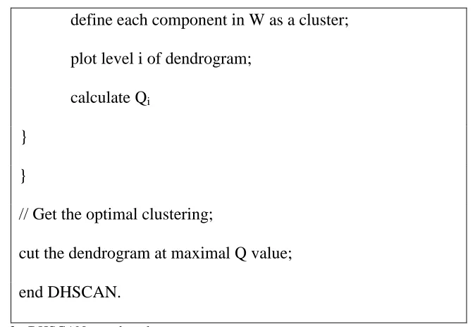
define each component in W as a cluster;
plot level i of dendrogram;
calculate Qi
}
}
// Get the optimal clustering;
cut the dendrogram at maximal Q value;
end DHSCAN.
Figure 2 - DHSCAN pseudocode
The authors point the ability to identify the optimal partition and the absence of
any input parameters as the advantages of their algorithm. None of the limitations or
drawbacks are mentioned as well as no complexity analysis is provided. Meanwhile the
long computation time is the main disadvantage of the algorithm as the demanding
operation of modularity calculation has to be applied every time the clustering structure
changes after the removal of certain number of edges.
II.1.3. AHSCAN
Some time after proposition of SCAN and DHSCAN an agglomerative version of the
hierarchical algorithm was introduced by the same research group [37]. AHSCAN uses
the same set of definitions as DHSCAN and the same core principle. In the beginning
every separate vertex forms its own cluster. The algorithm sorts edges in descending
order of edge structure value and removes them one by one, merging vertices (or clusters)
recalculated and the highest value, as well as corresponding clustering, is saved. ASCAN
does not require any input parameters, which is a definite advantage compared to SCAN.
For some reason, the authors decided to use Newman's modularity in order to identify the
best partition. Newman's modularity is 'well accepted by the research community' [37],
but as the authors mentioned in previous publications [36] and [14], it failed to identify
nodes of special importance: hubs and outliers. Thus AHSCAN in the form it is
introduced by the authors does not explicitly identify hubs and outliers.
The authors claim their algorithm to be linear with respect to the number of edges,
though complexity analysis is not provided in the paper, the result is just stated there. The
authors also suggest that AHSCAN to their knowledge 'is one of the fastest, if not only,
network clustering algorithms in literature' and the accuracy provided by the algorithm is
claimed to be 'quite competitive with one of the state-of-art agglomerative network
clustering algorithm, CNM, which has much higher complexity' [37]. CNM denotes
Clauset-Newman Modularity, which in turn is denoted as Fast Modularity in this work.
AHSCAN pseudocode is provided below and is taken from [37]:
Algorithm AHSCAN(G = <V, E>)
CALCULATE all κ(e) // e E
SET all κ(e) into P[]
SORT P[] in descending order
i := SIZE(E)
Max_Q := 0; // Max modularity
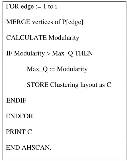
FOR edge := 1 to i
MERGE vertices of P[edge]
CALCULATE Modularity
IF Modularity > Max_Q THEN
Max_Q := Modularity
STORE Clustering layout as C
ENDIF
ENDFOR
PRINT C
END AHSCAN.
Figure 3 - AHSCAN pseudocode
II.1.4. Weighted graphs
All the algorithms mentioned above have one common property - they target unweighted
graphs. Every graph edge may have a positive number associated with it, which is usually
called edge weight or capacity. Weight/capacity might have different interpretations from
intensity of nodes interaction to the maximum amount of flow passing through the edge.
In any case edge weight encapsulates some valuable information about the graph and the
real-world structure it represents. When provided with a weighted graph, any of the
algorithms mentioned above will simply ignore the edge weights and will perform
clustering based on structural properties of the graph. While this might be acceptable in
certain cases, sometimes it is completely inadmissible. Some networks (graphs) simply
interconnected airports where edge weight corresponds to the distance between airports.
The fact of the possible connection between airports is, of course, of a crucial
importance, but without knowing the distance between them any operations on the graph
would not make much sense. Thus it is logical to expect the value of the edge weight to
influence the graph clustering.
Maximum flow-based algorithms may be considered an extension of minimum
cut algorithms for weighted graphs. The value of maximum flow between any two nodes
in graph is directly related to edge weights (or capacities). The cut definition for weighted
graphs is the same, but it gains an additional property - the value. The sum of edge
weights that constitute the cut is a cut value [16]. A cut with a minimum value is called a
minimum cut. Ford and Fulkerson in [16] showed that maximum flow between two nodes
is equal to the value of minimum cut, separating them. Based on this idea it is possible to
build a minimum cut tree. A tree is an unweighted connected graph without cycles.
Minimum cut tree of a graph G(V, E) is a tree that contains all the vertices of the graph G
and weighted edges connect vertices in a way that a path between any two vertices has a
capacity of a minimum cut.
One of well known maximum flow-based algorithms - minimum cut tree method
proposed by Flake et al. in [15] - is based on calculation of the minimum cut tree of the
graph using the algorithm proposed by Gomory and Hu in [18]. The clusters are achieved
by extending the original graph with an artificial sink t and connecting every existing
vertex to it by an edge with weight α. Using Gomory and Hu's algorithm the min cut tree
is then obtained. Removing the artificial node from the tree and getting the connected
Minimum cut tree clustering algorithm targets undirected weighted graphs. Being
a maximum flow based method it takes edge weights into consideration. Edge weights
have direct influence on the flow value, which in turn is used by clustering algorithm.
The algorithm requires an input parameter: the weight α of additional edges that connect
all the vertices to the artificial sink. Flake et al. analyze the influence of α value on the
clustering: when α is close to zero, the trivial cut, separating sink t from all other nodes in
the graph, will be minimum. If α in turn goes to infinity, the min cut tree turns into a star,
thus removing of a sink produces n singleton clusters, where n is the number of nodes in
the graph. In that way selection of α is important for the clustering result. Thus the
algorithm is capable of identifying isolated nodes, but it happens more as a by-product of
choosing inappropriate parameter value, so it is not likely that isolated vertices will be the
ones of some special role in the graph. In that way, mentioned algorithm has the same
drawbacks as most of methods mentioned before: inability to identify special nodes,
presence of input parameter, that might be hard for the user to determine.
It is worth mentioning that Fast Modularity algorithm, mentioned before as one of
the top clustering algorithms, originally targeting unweighted graphs, can be easily
extended to utilize edge weights. This procedure is described by Newman in [25].
II.2.Quality measurements
There are few ways of checking the quality of the achieved graph partition. When actual
partition is known a priory (if there exist known natural clusters in a form of divisions,
teams, groups, etc), achieved clustering can be compared to real clusters and thus quality
clustering, if existent, is rarely known a priory and consequently other methods should be
used to estimate the results. Quality assessment measures (functions) is another approach.
Such function takes graph partitioning (clustering) as input and calculates a value, usually
ranging from 0 to 1, that indicates the quality of partitioning. The higher the value, the
better the quality of the clustering.
Brandes and Erlebach in [2] describe the rules for such measurement design. The
process of clustering usually focuses on two main properties: intra-cluster density and
inter-cluster sparsity. Thus a good quality measurement function should take them both
into consideration. Denoting density inside clusters with f and sparsity between clusters
with g, Brandes and Erlebach define the general look of such function by the formula:
(9)
where A(G) is the set of all possible partitions. In this way the function achieves its
maximum value of 1 for the 'extremely' fitting clustering and the minimum value of 0 in
case of absence of meaningful clusters or totally random.
II.2.1. Newman's modularity
The most popular and well accepted by the researchers quality measurement is
modularity proposed by Newman and Girvan in [27]. To calculate the modularity one
needs to construct symmetric k by k matrix e, where k is number of clusters. Diagonal
elements eii of the matrix contain the fraction of graph edges that connect vertices in i-th
cluster, while the rest matrix elements eij contain the fraction of edges connecting i-th
(10)
produces the fraction of intra-cluster edges of the graph. Matrix trace corresponds to
density f in Brandes and Erlebach work [2] and is not sufficient for adequate clustering
assessment by itself, as a single cluster containing all graph vertices will result in
maximum trace value equal to 1 [27]. To include sparsity g in the estimate the 'row (or
column) sums' are introduced:
(11)
that represent the fraction of edges connecting to the vertices in cluster i. Thus the authors
define modularity:
(12)
where denotes the sum of the elements of the matrix e [27].
II.2.2. Novel Similarity-Based Modularity
Feng et al. in [14] criticize Newman's modularity. The authors claim that Newman's
modularity works very well with clear clustering structure, where the inter-cluster
connections are sparse. But modularity method fails to process effectively partitions with
'hub' and 'outlier' types of vertices that do not belong to any particular cluster or produce
singleton clusters. To address this issue the authors propose similarity-based modularity
for the graph V:
(13)
where
, (15)
, (16)
NC is number of clusters, - total similarity of vertices in i-th cluster, - total
similarity between any vertices in the graph and vertices in cluster i, TS - total similarity
between any two vertices in the graph; - structural similarity of vertices u and v,
defined before.
Feng et al. claim that their similarity-based modularity produces better results in
graphs with 'more confused' sub-graph structure, including vertices of special importance:
hubs and outliers [14].
II.2.3. Performance
Performance is another quality measure that combines measures for inter-cluster sparsity
g and intra-cluster density f. Performance was first proposed by Iverson in [21] and later
adapted by Knuth in [23]. Performance counts particular node pairs. As for the density f,
it consists of 'correctly' classified pairs that belong to the same cluster and are connected
by an edge; the other case, intra-cluster sparsity g consists of 'nonexistent edges' - pairs
that belong to distinct clusters and are not connected by an edge - [2]:
(17)
(18)
where C is clustering of the graph G(V, E), - the set of intra-cluster edges.
Calculating maximum of f + g is NP-hard [29], but obviously is has n(n - 1) as the
upper bound (where n is the number of nodes), simply because there are n(n - 1) possible
Brandes and Erlebach in [2] provide the derivation of the formula for performance
calculation:
(19)
where m is the number of edges in the graph, and m(C) is the number of
intra-cluster edges in the partition.
II.3.Graph Generators
Random or generated graphs are often used in different experiments that involve graphs
and graph clustering is not an exception. Real world datasets might be hard to access
and/or require significant effort to parse and transform to graph form. Therefore graph
generators provide relatively easy solution. Properly generated graph will have (or at
least will be expected to have) predefined community structure and thus may be used to
validate clustering algorithms. Also many years of study reveal a fact that real world
graphs follow certain patterns that keep reoccurring in various fields of science. Surveys
like the one by Costa et al. [7] list these patterns.
II.3.1. Planted l-partition model
A famous graph-generating framework was proposed by Girvan and Newman and
originally used in [17], being applied afterwards in many research papers: [27], [26] and
others: [19]. This framework is a special case of so-called l-partitioned model originally
proposed by Condon and Karp in [6]. L-partitioned model has predefined community
model has n = g * l vertices, where l is number of clusters with g vertices in each.
Vertices are connected with probabilities pin for intra-cluster edges and pout for
inter-cluster ones. The average degree can be calculated using the following formula:
(20)
Community structure in the graph is present when pin > pout (which means that
intra-cluster density is higher than inter-intra-cluster density).
Girvan and Newman framework is a special case of planted l-partition model with
l = 4 and g = 32 (number of vertices in graph is 128) and average degree k equal to 16.
The graph generator has a parameter that specifies the level of intra-cluster density: the
average number of inter-cluster edges zout for every vertex (vertex outer degree). Thus the
distinguishable community structure can be obtained for zout values up to 8. Various types
of community structure are depicted on the Figures 4 to 6:
Figure 5 - Community structure with 4 inter-cluster edges per node
Figure 6 - Community structure with 6 inter-cluster edges per node
Normally it is hardly possible to identify community structure with zout more or
equal to 8.
II.3.2. Preferential attachment
In [1] Barabasi, studying real-world networks (like genetic networks or World Wide
gaining new vertices, they (new vertices) are more likely to become connected to a high
degree vertex. Barabasi proposed a method for graph generation that begins having a
small number of vertices and adds a new one (as well as specified number of edges) at
every time step probability. Edges are attached to existing vertices in order to incorporate
preferential attachment principle: the probability to be connected to the existing vertex i
is:
(21)
where |E| is the number of existing edges in the graph.
The developers of an open source JUNG graph library implemented this graph
generating method and included it in their library with some modifications. They noticed
that the formula x always produces zero probability for an isolated vertex. Thus to "give
each existing vertex a positive attachment probability" developers utilized the following
formula:
(22)
where |V| is the number of vertices already existent in the graph.
II.3.3. Power laws
Another important feature found for web-graphs in the same work [1] by Barabasi and
Albert is power-law degree distribution, which happens to be a consequence of
preferential attachment and incremental growth. Due to Barabasi and Albert power law
degree distribution consists in the fact that probability of a vertex in the graph with a
(23)
Eppstein and Wang in [11] suspect power law degree distribution to be an
ubiquitous property of real-world graphs. At least the authors state that it is present in
epidemiology, population studies, genome distribution, etc. The authors propose a graph
generation method that does not require incremental growth, instead it utilizes and evolve
an existing graph according to a Markov process. The iterative algorithm is provided
below:
1. Pick a random vertex v with non-zero degree.
2. Pick an edge (u, v) from the graph at random
3. Pick another random vertex x.
4. Pick a vertex y not equal to x with a proportional to degree probability.
5. If an edge (x, y) does not exist in the graph, remove the edge (u, v) and add
edge (x, y).
II.3.4. Community structure
Defining community as a subgraph where vertices are closer to each other (in terms of
similarity functions) than to the ones in other subgraphs, the fact that community
structures are ubiquitous in real world graphs probably can be considered indirectly
proved by variety of clustering algorithms existent today. In social networks community
structure reveals itself by a simple pattern: individuals usually have more connections to
other members of the same community than to ones from other groups [22]. A number of
metrics to measure the clumpiness of a graph was proposed. One of the most basic and
the graph [24], [3], but there also exists an alternative definition of a clustering
coefficient of a single vertex provided by Watts and Strogatz in [33]. The latter is of a
particular interest for us, thus we will explain it here in more detail.
Clustering coefficient for a vertex i is defined as
(24)
where ki is the number of vertex i neighbours and ni is the number of edges between the
neighbours. The central node X on Figure 7 has 6 neighbours, and there are 5 edges
between the neighbours (not including the edges incident to X). Thus local clustering
coefficient of the node X is 5/6.
CHAPTER III
DESIGN AND METHODOLOGY
III.1.Extended structural similarity
Among the variety of existing clustering algorithms SCAN and other based on it
algorithms (DHSCAN and AHSCAN) distinguish themselves as they exhibit some
important features: the ability to identify nodes of a special interest - hubs and outliers,
and to a greater extent - focus on neighbourhood for identifying clusters. This 'social'
aspect, as all three algorithms are based on the structural similarity - the value derived
from the neighbourhood structure, the idea of using information about neighbours to
make a decision about clustering, makes these algorithms particularly promising for the
sake of Social Network Analysis. Intuitively this property seems to have a great validity
in real world social networks. In the famous experiment by Travers and Milgram in [32]
people had to send a chain letter to reach a random person of interest. Thus people used
only their 'direct neighbourhood' - only people they knew - to send a letter intended to
someone they do not know. The experiment revealed the concept of six degrees of
separation: the average length of chain was six, which is considered a very small number
taking into the account the size of population affected. This experiment shows the
importance of the neighbours in the social graph. Thus the idea of using this information
for clustering seems to us extremely valuable.
No other known clustering algorithms possess both of these features: usage of
neighbourhood information and ability to identify nodes of special importance. On the
other hand, a serious limitation of SCAN based algorithms is the fact that they target
chapter II. To avoid this limitation we introduce the weighted versions of SCAN and
SCAN-based algorithms. These algorithms use modified structural similarity that
incorporates edge weights.
In [4] a weighted version of SCAN which allows to overcome the mentioned
limitations was already introduced. However, the new algorithm was just presented, and
was never compared to any other existing clustering algorithm. Moreover the extension
created another drawback. The proposed algorithm used slightly modified formula for
structural similarity:
(25)
where is a weight of the edge connecting vertices and .
Adopting edge weights, this formula at the same time introduces a limitation:
similarity between vertices that are not connected by an edge turns to zero, which
significantly limits the potential of the mentioned social structure concept based on
neighbourhood.
Indeed vertices V1 and V8 on figure 4 are not connected on the picture, but if we
calculate the structural similarity between them, we will get rather high value of 0.857,
which would normally mean that these two vertices are very similar.
In this work we propose modifications to Weighted SCAN in order to improve its
ability to detect clusters and apply the same approach to derived DHSCAN and ASCAN.
To overcome the limitations of Chertov's approach we introduce extended
structural similarity defined like this:
(26)
where is the maximum weight in the graph or
(27)
where is normalized weight of the edge connecting vertices and . Thus a
graph needs to be 'normalized' before weighted SCAN can be applied to its edge weight
values.
The base of the similarity between two vertices remains the same - similarity of
people sharing many friends, but not knowing each other (not being connected by an
edge in the graph) remains the same, while the existence of the connection (an edge)
between them only increases the value of structural similarity.
Thus all the algorithms (SCAN and derived from it DHSCAN and ASCAN)
remain the same, except the formula of structural similarity used at many steps of the
algorithms. The change in the absolute value of the similarity affects SCAN, but none of
its derivatives as they use comparative value of similarity and similarity of almost every
pair of vertices is affected. In case of modified version of SCAN adjustment of ε
Since now we will not go back to unweighted versions of the algorithms and by
SCAN, DHSCAN and AHSCAN we will denote weighted versions of these algorithms,
which use the aforementioned approach (formulas 26 and 27) to structural similarity
(unless mentioned explicitly).
III.2.Clustering quality assessment
For quality assessment of the clustering result, we use adapted Newman's modularity and
Similarity-Based Modularity, mentioned in chapter II.
III.2.1. Newman's modularity
Modularity, introduced by Newman and Girvan in [27] targets unweighted graphs.
Matrix e, used in calculations, is populated with regard to the number (and fraction) of
edges connecting vertices in the graph, vertices in the same cluster and vertices in
different clusters. In [25] Newman describes the idea of its extension: using actual edge
weights instead of counting the number of edges. The same formula for modularity
calculation is used:
(28)
Instead of number of edges in the graph now the total 'graph weight' is calculated - the
sum of all edge weights in the graph. For diagonal elements of matrix e (eii) the sum of
edge weights connecting vertices in cluster i and then find the fraction of this sum weight
in the 'graph weight' is computed. Similarly for regular elements eij the fraction of edge
weights connecting vertices in cluster i to vertices in cluster j is calculated.
(29)
where A is adjacency matrix of the graph, function is defined like:
(30)
m is the number of edges in the graph, ki - is the degree of vertex i.
For weighted networks, matrix A turns into an extended adjacency matrix, where
corresponds to the weight of the edge connecting vertices i and j, degree ki is defined
according to the formulas:
(31)
(32)
Non zero values of modularity 'indicate deviations from randomness', while
values around 0.3 or more usually correspond to good partitions. Maximum possible
modularity value is 1 [25].
III.2.2. Similarity-based modularity
Similarly to Newman's modularity similarity-based modularity was proposed to measure
the quality of unweighted graph clustering. As mentioned in chapter II, the value of
similarity-based modularity is calculated based on structural similarity. SCAN, DHSCAN
and AHSCAN are also based on the notion of structural similarity. Analogously to
extending the clustering algorithms by making them use weighted structural similarity,
we substitute similarity-based modularity with its extended weighted version:
(33)
, (34)
, (35)
, (36)
NC is number of clusters, - total extended similarity of vertices in i-th cluster, -
total extended similarity between any vertices in the graph and vertices in cluster i, TS -
total extended similarity between any two vertices in the graph; - extended
structural similarity of vertices u and v, defined before.
The table 1 provides the comparison of the values of the unweighted and weighted
Qs for different partitions of the graph of the figure 10.
Clustering structure Unweighted Qs Weighted Qs
All vertices in one cluster 0 0
{a }, {b, c, d}, {f, e, g}, {h} 0.22727 0.22052
{a, b, c, d}, {e, f, g}, {h} 0.21491 0.21091
{ a b c d }{ e f g h } 0.22650 0.22415
{f e a g }{h }{b d c } 0.23582 0.23591
{b, c, d},{a, e, f, g, h} 0.23916 0.23985
{a},{b, c, d},{e, f, g, h} 0.23886 0.23376
Table 1 - Weighted and unweighted structural similarity-based modularity.
These values are a little different from the results published by Feng et al. in [14]
where the similarity-based modularity was first introduced. Feng et al. had the maximum
modularity value for {a},{b, c, d},{e, f, g, h}, while {b, c, d},{a, e, f, g, h} had a little
less. We have the opposite situation, though the values are very close to each other. This
gives rise to questioning the validity of similarity-based modularity. After contacting the
authors we resolved ambiguity in modularity calculation and multiple checks of the
calculation algorithm did not identify any reason for us having different values of the
quality functions. However, introducing weights into the computation does not
significantly change the relative function values. The best identified partition is still the
same.
If we increase the weight of one single edge fh to make it five times stronger than
all other edges (to keep the values in [0, 1] range we also decrease values of other edges),
we will be able to notice some changes in the weighted similarity-based modularity
Figure 10 - Graph with different weight distribution
The weight of an outlier edge connecting g and f is 5 times bigger - we see
tendency to put h into an adjacent cluster.
Clustering structure Q unweighted Weighted Q
All vertices in one cluster 0 0
{a }, {b, c, d}, {f, e, g}, {h} 0.22727 0.20852
{a, b, c, d}, {e, f, g}, {h} 0.21491 0.20195
{ a b c d }{ e f g h } 0.22650 0.23008
{f e a g }{h }{b d c } 0.23582 0.22302
{b d c }{f e a g h } 0.23916 0.23833
{a }{b d c }{f e g h } 0.23886 0.17328
Table 2 - Weighted and unweighted similarity-based modularity values
The observed behaviour can be considered rather strange, but we can still see the
tendency to identify hubs and outliers: the absolute value of the partitions with isolated
vertex h went noticeably down.
It is worth to be noted again, that DHSCAN and AHSCAN, being developed by
clustering quality measurements to find an optimal solution. It might imply that
similarity-based modularity is not as good as it was thought to be originally. We are
going to check it in our experiments.
III.2.3. Performance
For weighted performance we will use one of the variations included in [2], where
is sum of weights of intra-cluster edges:
(37)
and is maximum possible weight of non-existent inter-cluster edges:
(38)
where C is clustering of the graph G(V, E), and M is some meaningful maximum edge
weight.
The value of M may introduce some disturbance into calculation, if weights are
not uniformly distributed - in other words the presence of a single extremely large edge
weight will influence the performance significantly, disrupting 'the range aspects' of the
quality measurement [2].
The obvious drawback of this approach is neglecting the weight of inter-cluster
edges. The following modification can be used:
(39)
where
(40)
and is a set of inter-cluster edges in partition C.