Numerical simulation of flow surrounding a thermoacoustic stack:single-stack against double-stack plate domain

(1)

78: 8–4 (2016) 119–125 | www.jurnalteknologi.utm.my | eISSN 2180–3722 |

Jurnal

Teknologi

Full Paper

NUMERICAL

SIMULATION

OF

FLOW

SURROUNDING A THERMOACOUSTIC STACK:

SINGLE-STACK AGAINST DOUBLE-STACK PLATE

DOMAIN

Normah Mohd-Ghazali, Liew Kim Fa

Faculty of Mechanical Engineering, Universiti Teknologi

Malaysia, 81310, UTM Johor Bahru, Johor, Malaysia

Article history

Received

1 January 2016

Received in revised form

18 May 2016

Accepted 15 June 2016

*Corresponding author

[email protected]

Abstract

Over the last few decades, numerical simulation has fast become an effective research tool in analyzing internal and external fluid flow. Much of the unknowns associated with microscopic bounded and unbounded fluid behavior generally not obtainable via experimental approach can now be explained in details with computational fluid dynamics modeling. This has much assist designers and engineers in developing better engineering designs. However, the choice of the computational domain selected plays an important role in exhibiting the correct flow patterns associated with changes in certain parameters. This research looked at the outcomes when two computational domains were chosen to represent a system of parallel stack plates in a thermoacoustic resonator. Since the stack region is considered the “heart” of the system, accurate modeling is crucial in understanding the complex thermoacoustic solid-fluid interactions that occur. Results showed thatalthough the general flow pattern and trends have been produced with the single and double plate stack system, details of a neighboring solid wall do affect the developments of vortices in the stack region. The symmetric assumption in the computational domain may result in the absence of details that could generate an incomplete explanation of the patterns observed such as shown in this study. This is significant in understanding the solid-fluid interactions that is thermoacoustic phenomena.

Keywords: Computational domains, parallel stack plates, thermoacoustic resonator, vortices, solid-fluid interactions

Abstrak

Sejak beberapa dekad yang lalu, simulasi berangka pantas menjadi satu alat penyelidikan yang berkesan dalam menganalisis aliran bendalir dalaman dan luaran. Banyak yang tidak diketahui berkaitan kelakuan bendalir mikroskopik disempadani dan tidak disempadani yang tidak diperolehi melalui pendekatan eksperimen sekarang dapat dijelaskan secara terperinci dengan model pengiraan dinamik bendalir. Ini telah banyak membantu pereka dan jurutera dalam membangunkan rekabentuk kejuruteraan yang lebih baik. Walaubagaimanapun, pilihan domain pengiraan dipilih memainkan peranan yang penting dalam mempamerkan corak aliran yang betul dikaitkan dengan perubahan dalam parameter tertentu. Kertas kerja ini membincangkan hasil dari dua domain pengiraan dipilih untuk mewakili sistem plat timbunan selari dalam resonator termoakustik. Oleh kerana kawasan timbunan dianggap sebagai "jantung" sistem, pemodelan tepat adalah penting dalam memahami interaksi pepejal-cecair termoakustik yang berlaku. Hasil kajian menunjukkan bahawa walaupun corak aliran serta trend telah dihasilkan dengan sistem plat timbunan satu dan dua, butir-butir dinding pepejal jiran jelas memberi kesan kepada perkembangan pusaran di rantau timbunan. Andaian simetri dalam domain pengiraan boleh menyebabkan ketiadaan butir-butir yang boleh menjana penjelasan tidak lengkap corak yang diperhatikan seperti yang ditunjukkan dalam kajian ini. Ini penting dalam memahami interaksi pepejal-cecair fenomena termoakustik.

Kata kunci: Domain pengiraan, plat timbunan selari, resonator termoakustik, pusaran, interaksi pepejal-cecair

(2)

1.0 INTRODUCTION

Although the first successful thermoacoustic refrigerator was completed about thirty years ago [1], much is still unknown about the thermoacoustic phenomena which occurs due to the fluid-solid interactions of oscillating fluid particles passing over solid walls. The flow behavior affects the degree of cooling attainable and studies have been completed experimentally and numerically to investigate the effects of the solid walls; thickness and separation gap. However, since the performance of the thermoacousticrefrigerator to date is still low, particularly the standing wave type, research continues to better understand the flow pattern surrounding the stack plate, the “heart” of the system. Experimental techniques with flow visualization such as the holographic interferometry, laser Doppler anemometer (LDA) and particle image velocimetry (PIV), though non-intrusive, limit the stack geometry design and thickness [2-7]. The experimental set-ups involved larger than that recommended plate thickness and separation gap in order to generate acceptable and significant visuals to be captured by the related measuring apparatus. In particular, the desired stack plate thickness should be as thin as possible to avoid a vertical temperature gradient across the plate thickness.

The first numerical simulation of the thermoacoustic effects was by Cao et al. [8] but the study with a negligible thickness plate assumed the standing wave as a priori. The first simulation on the whole resonator where the stack is encased was probably by Mohd-Ghazali [9], where many complex behaviors were reported as the acoustics were generated and progressed. Zoontjenset al. [10] utilized a commercial CFD package, FLUENT, to model the flow behavior near a single plate. Experimental and numerical studies have shown streaming effects near the stack which could be the reason for the low performance of the thermoacoustic refrigerator [2-7, 9-12]. This and the presence of vortices removed the kinetic energy otherwise absorbed by the stack for the heat transfer processes. These studies on single- and two-plate stack region have not focused onthe differences resulted from the choice of the computational domain where the general macroscopic behavior of the vortices and streaming are always observed. Thus, this study has been undertaken to look at the flow surrounding a single-plate and a double-plate stack to identify if there is any difference that exist in the development of the streaming effects and vortices.

2.0 THEORETICAL FORMULATION

The working fluid in the present model is air, assumed as an ideal Newtonian gas operating at atmospheric pressure and 298K. The unsteady flow considered is two-dimensional, inviscid and incompressible with the absence of any external forces. The governing

equations for the fluid are the conservation of mass, momentum, and energy, given by,

𝜕𝑝/𝜕𝑡 + ∇. (𝜌𝑢)= 0 (1)

𝜌𝐷𝒖_𝐷𝑡= −𝛁𝑝 (2)

𝜌𝑐𝑝𝐷𝑇_𝐷𝑡= 𝛁 ∙ (𝑘𝛁𝑇) +𝐷𝑝_𝐷𝑡 (3)

where ρ, cp, k, p, T, and t each stands for the density,

constant pressure specific heat, pressure, temperature, and time, and u represents the velocity vector. Together with the ideal gas equation,

𝑝 = 𝜌𝑅𝑇 (4)

and an unsteady conduction within the stack gives,

𝜌𝑐𝑝𝐷𝑇_𝐷𝑡= 𝛁 ∙ (𝑘𝛁𝑇) (5)

Due to the compression and expansion of the gas particles, the density, pressure, velocity, and temperature are defined as [10],

𝜌 = 𝜌𝑚+ 𝜌∗ (6)

𝑝 = 𝑝𝑚+ 𝑝∗ (7)

𝒖 = 𝒖𝑚+ 𝒖∗ (8)

𝑇 = 𝑇𝑚+ 𝑇∗ (9)

Equations (4) and (6) through (9) are substituted into

equations (1), (2), (3) and (5).The terms pm,ρm and Tm

are the constants which are 101.325kPa, 298K and

0.1637 kg/m3_{respectively. They are the mean}

operating conditions based on the work of Mohd-Ghazali [9]. The p*, ρ* and T* are the fluctuating parts to be determined.Subsequently upon simplifications, all the fluctuating terms hereforth are used without the “asterick”, the unknowns. The Boussinesq approximation is applied which states that the change in the density

can be neglected which is ρ= ρm. Details of the

derivation may be found in Mohd-Ghazali [9] as well as in Liew [13].

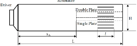
The physical domain of the thermoacoustic resonator is shown schematically in Figure 1. The overall length of

the resonator, L, is taken to be 0.635m, which is λ/4, 

(3)

Figure 1 Physical domain of the thermoacoustic resonator

The computational domain of a single plate and double plate configurations modeled in this study is shown in Figure 2 and Figure 3 respectively. The initial

conditions (at time, t = 0) are 𝑢 = 0, 𝑣 = 0 and 𝑇 = 𝑇𝑚 for

all computational domains. These mean that the fluid particles are stationary with a mean temperature in the

resonator. The boundary conditions of the

computational domain are set-up such that a quarter wavelength standing wave is set-up in the computational domain:

AC : 𝑢 = 𝑢𝑜cos(𝑘𝑥𝐴) sin(𝜔𝑡) , 𝑣 = 0, 𝑇 = 𝑇𝑚

BD : 𝑢 = 0, 𝑣 = 0,𝜕𝑇_𝜕𝑥= 0

EF : 𝑢 = 0, 𝑣 = 0,𝜕𝑇_𝜕𝑥= 𝛾𝛼(∇2_𝑇)

AB and CD : _𝜕𝑦𝜕𝑢 = 0, 𝑣 = 0,𝜕𝑇_𝜕𝑦= 0

Figure 2 Computational domain of a single plate configuration

Figure 3 Computational domain of a double plate configuration

The model follows that of to Tijani’s physical system [15], the working gas used being Helium at the operating frequency of 400Hz. The drive ratio, Dr, which is defined as the ratio of pressure amplitude to the system pressure is set at 0.5%. With the relation of velocity amplitude to the pressure amplitude, 3m/s is

determined to be used as the velocity amplitude, 𝑢𝑜.

The length of the stack and the stack separation are 95mm and 2mm respectively.

3.0 NUMERICAL FORMULATION

The second-order partial derivatives are converted into algebraic forms using the second-order finite difference

scheme for each dependent variable, , and

independent variable, s, 𝜕2_𝜃

𝜕𝑠2 ≅

𝜃_𝑖+1,𝑗𝑘 _−2𝜃 𝑖,𝑗𝑘+𝜃𝑖−1,𝑗𝑘

(∆𝑠)2 (10)

where may represent the velocity, pressure, and

temperature, the unknowns. The subscripts i and j refer to the axial and vertical spatial difference while k refers to the temporal difference. The first-order partial derivative is represented by,

𝜕𝜃

𝜕𝑠≅

𝜃_𝑖+1,𝑗𝑘 _−𝜃 𝑖−1,𝑗𝑘

2∆𝑠 (11)

and the mixed derivative by, 𝜕2_𝜃

𝜕𝑠1𝜕𝑠2≅

𝜃_{𝑖+1,𝑗+1}𝑘 _−𝜃

𝑖+1,𝑗−1𝑘 −𝜃𝑖−1,𝑗+1𝑘 +𝜃𝑖−1,𝑗−1𝑘

4∆𝑠1∆𝑠2 (12)

withs1 and s2 for x and y respectively. As for the value at the boundaries, second order forward difference is used at the x = 0 and y=0 and second order backward

difference is used at 𝑥 = 𝐿and x = h + d, which are,

𝜕𝜃

𝜕𝑠≅

−3𝜃𝑖,𝑗𝑘+4𝜃𝑖+1,𝑗𝑘 −𝜃𝑖+2,𝑗𝑘

(∆𝑠)2 (13)

𝜕𝜃

𝜕𝑠≅

3𝜃_𝑖,𝑗𝑘_−4𝜃 𝑖+1,𝑗𝑘 +𝜃𝑖+2,𝑗𝑘

(∆𝑠)2 (14)

For two-dimensional computational domain simulation,

the grid spacing for ∆𝑥 and ∆𝑦 are 0.0005m and 0.0002m

respectively. The time step,∆𝑡 is 31.25µs in order to make

explicit equations stable since the period of a cycle is 2.5ms. Four cases are investigated as shown in Table 1.

Table 1 Cases investigated for different computational domain

Case Number of

plates spacing Plate thickness Plate

1a 1 2 0.4

1b 2 2 0.4

2a 1 2 0.8

2b 2 2 0.8

4.0 RESULTS AND DISCUSSION

Figure 4 shows the comparison made between the one-dimensional inviscid and viscous simulation that exhibits no significant difference. A quarter-wavelength standing wave is progressively being developed with time in the resonator.

(4)

Thus, simulation for the two-dimensional computational domain is continued under the inviscid assumption. Outcomes of the simulation for the single- and two-plate stack system are shown in Figures 5 through 10, captured at different time to show the temporal development of the velocity profiles.

(a)

(b)

Figure 5 Case 1 -Vector plot and streamline at 7T/16 for a (a) single-plate, and (b) two-plate stack

(a)

(b)

(a)

(b) Figure 7 Case 1 -Vector plot and streamline at 9T/16 for a (a)

single-plate, and (b) two-plate stack

(a)

(b)

Figure 8 Case 1 -Vector plot and streamline at12T/16 for a (a) single-plate, and (b) two-plate stack

(a)

(b)

(a)

(b)

(5)

before the stack plate(s) at and before the half cycle, 8T/16, disappeared at 9T/16, appearing again later. However, the “purging” of the elongated vortices between the two plates is only clear in the two-plate computational domain of Figures 6b, 7b, and 8b. This progress is not discerned in Figures 6a, 7a, and 8a. The flow pattern is symmetric with respect to the system centerline. In particular, the existence of a neighboring plate affects the behavior of the flow close to the plate edges. Simplification through a symmetric assumption at the plate centerline in this case would result in some

missing understanding of the thermoacoustic

phenomena of heat transfer by the oscillating fluid particles. As seen here in Figure 7 and Figure 8, the adjacent plate resulted in a different velocity and vector profiles between the single-plate and double plate stack system.

Figures 11 through 16 shows that the flow patterns are asymmetrical along the plate centerline, in this case a thicker plate than that in Figures 5 through 10 with double the grid size. It seems that with a thicker solid stack domain shows a more obvious difference between the single-plate and double-plate stack computational domain as seen in Figures 11 and 12. There are missing details in Figures 13(a) and 16(a) which are observed in 13(b) and 16(b) in-between the plates. It is believed that the effects may be intensified as time progresses in the simulation and much more details could be missed.

(a)

(b)

(a)

(b)

(a)

(b)

(a)

(b)

(6)

(a)

(b)

(a)

(b)

The simulation results presented here have shown the importance of selecting the correct computational domain to represent the physical phenomena that is to be modelled. For certain selected domains, the overall effects may be observed i.e. macroscopically, but certain cases such as in this study of thermoacoustic phenomena, details essential towards explaining the complex behaviour may be missed. As such, inclusion of the viscous effects in future simulation is encouraged to investigate the boundary layer effects next to the solid walls of the plate, which have generally been described in Mohd-Ghazali [9].

5.0 CONCLUSION

Numerical simulation of the flow surrounding a single-plate and two-single-plate stack region has been completed to compare the effects of the selection of a computational domain in the thermoacoustic stack region. The choice of a symmetric line is particularly

important when many solid walls are present in the direction of the oscillating fluid flow. Results showed that although the general flow pattern and trends have been produced with the single and double plate stack system, details of a neighboring solid wall do affect the developments of vortices in the stack region. This is significant in understanding the solid-fluid interactions that is thermoacoustic phenomena.

Acknowledgement

The authors wish to thank UniversitiTeknologi Malaysia for the Research University Grant (GUP) Vote number O8H29 for the funding to assist in this research.

References

[1] Hofler, T.J. 1986.Thermoacoustic Refrigerator Design and

Performance. PhD Thesis, University of California, San Diego.

[2] Wetzel, M. and Herman, C. 2000. Experimental Study f

Thermoacoustic Effects on a Single Plate Part I: Temperature Fields. Heat and Mass Transfer.36(1):7-20.

[3] Trávníček, Z., Wang, A.B., Lédl,V., T. Vít, Chen, Y.C. and

Maršík, F. 2013. Holographic-Interferometric and

Thermoanemometric Study of aThermoacoustic Prime Mover. Journal of Mechanics. 29: 59-66.

[4] Bailliet, H.,Lotton, P., Bruneau,M., Gusev, V.,Valière, J.C.

andGazengel, B. 2000.Acoustic Power Flow Measurement in a Thermoacoustic Resonator by Means of Laser Doppler

Anemometry (L.D.A.)and Microphonic

Measurement.Applied Acoustics. 60(1):1-11.

[5] Thompson, M.W., Atchley, A.A. 2005. Simultaneous

Measurement of Acoustic and Streaming Velocities in a Standing Wave Using Laser Doppler Anemometry. J

AcoustSocAm. 117(4):1828–1838.

[6] Blanc-Benon, P., Besnoin, E.,andKnio, O. 2003. Experimental

and Computational Visualization of the Flow Field in a Thermoacoustic Stack. Mecanique. 331:17-24.

[7] Zhang, D.W., He, Y.L., Yang, W.W., Wang, Y. and Tao, W.Q.

2013. Particle Image Velocimetry Measurement On The Oscillatory Flow At The End Of The Thermoacoustic Parallel Stacks. Applied Thermal Eng. 51(1-2): 325-333.

[8] Cao, N. Olson, J.R., Swift, G.W., and Chen, S. 1996. Energy Flux

Density in aThermoacoustic Couple. The Journal of

Acoustical Society of America. 99(6): 3456-3464.

[9] Mohd. Ghazali, N. 2001. Numerical Simulation of Acoustics

Waves in a Rectangular Chamber. Ph.D. thesis Univ. of New

Hampshire.

[10] Zoontjens, L., Howard, C.Q., Zander, A.C. and Cazzolato, B.S.

2009. Numerical Study of flow and Energy Fields in Thermoacoustic Couples of Non-Zero Thickness. International

Journal of Thermal Science. 48(4):733-746.

[11] Abd El-Rahman, A.I. and Abdel-Rahman, E. 2013.

Computational Fluid Dynamics Simulation of a

Thermoacoustic Refrigerator. Journal of Thermophysics and

Heat Transfer. 28(1): 78-86.

[12] Liew, K.F. and Mohd-Ghazali, N. 2015. Simulation of the Flow

and Temperature Development Around the Stack Plate in a Thermoacoustic Resonator at Various Thickness and Separation Gap. Accepted for publication Int. Journal of

Tech.

[13] Liew, K.F. 2015. Simulation of the Fluid Flow around the Stack

Unit in a Thermoacoustic Resonator. Undergraduate Thesis Universiti Teknologi Malaysia.

[14] Setiawan, I., Utomo, A.B.S., Katsuta, M. and Nohtomi, M. 2013.

(7)

Thermoacoustic Refrigerator. Paper Presented at the Journal