PyNTA: An Open Source Software Application for
Live Particle Tracking
Aquiles Carattino1 , Allard P. Mosk1 , and Sanli Faez1,†
1Nanophotonics, Debye Institute for Nanomaterials Research, Utrecht University
* † Correspondence: [email protected]
Simple Summary: A new open-source software package for live particle tracking provides the possibility of intensive data processing while acquiring images at the highest possible readout speed with a camera.
Abstract: We introduce PyNTA, a modular instrumentation software for live particle tracking. By using the multiprocessing library of Python and the distributed messaging library pyZMQ, PyNTA allows users to acquire images from a camera at close to maximum readout bandwidth while simultaneously performing computations on each image on a separate processing unit. This publisher/subscriber pattern generates a small overhead and leverages the multi-core capabilities of modern computers. We demonstrate capabilities of the PyNTA package on the featured application of nanoparticle tracking analysis. Real-time particle tracking on megapixel images at a rate of 50 Hz is presented. Reliable live tracking reduces the required storage capacity for particle tracking measurements by a factor of approximately 103, as compared with raw data storage, allowing for a virtually unlimited duration of measurements.
Keywords: video microscopy, imaging, automated data acquisition, nanoparticle tracking, measurement embedded applications, open-source software
1. Introduction
Experiments in STEM fields increasingly rely on digital data acquisition and storage. While computation power has grown tremendously, the increasing complexity and bandwidth of sensory equipment are for some experiments outpacing the storage capacity and bandwidth. One widely used example is video microscopy that usually comes with a high rate of data generation. In most experiments, the actual required information is not the data contained in each pixel of the raw images, but specific features in the frame. While several approaches have been introduced for industrial applications, these customised solutions are not available to researchers that perform small-scale table-top experiments. As a result, data acquisition and data analysis are mostly performed on separate stages (for example see Chenouardet. al.[1] and the references there-in). This procedure is time consuming and a major limitation on the experimental workflow because real-time feedback and adjustment is not possible [2]. Moreover, when working with videos, every new frame needs to be stored. Since the amount of memory on the computer and the writing speed on hard drives is limited, the experiments face a limitation caused by storage capacity and bandwidth, rather than by computational power.
Here, we introduce PyNTA, an open-source software package written in Python, that allows acquiring images from a camera at maximum bandwidth while simultaneously performing computations on each image on a separate processing unit. The program generates real-time results and therefore only the necessary processed information needs to be stored. The graphical user interface and direct control on the measurement instrument are built into the package, empowering users to act on the available data during the measurement. Here we demonstrate the capabilities of the
PyNTA package by focusing on nanoparticle tracking analysis (NTA) as a widely used application. We emphasise that the approach can be adapted and extended to any other instrumentation software.
PyNTA is released as open source with a GPLv3 license, and can be installed on any PC running Windows, Linux, or MacOS operating systems. Contribution guidelines are provided to enable other developers to easily extend or add new features to the program.
2. Nanoparticle tracking analysis
Measuring the size of objects with a diameter below the diffraction limit requires dedicated techniques. Electron microscopy gives access to very accurate results but requires a high investment and is very time-consuming. Optical ensemble measurements such as dynamic light scattering (DLS) are more affordable but best suited for relatively homogeneous samples. The results of inhomogeneous samples will be dominated by the properties of brighter particles, even if they are not statistically more abundant [3]. Single-nanoparticle tracking analysis (NTA) is a video microscopy technique that can be applied to samples with heterogeneous particle sizes at a fraction of the cost of using electron microscopy.
NTA relies on correlating the random motion of the particles to their diameter through the use of the Stokes-Einstein equation:
D= kBT
3πηd , (1)
whereDis the diffusion coefficient,kBthe Boltzmann constant,Tthe temperature,ηthe viscosity of the medium anddthe particle diameter. In order to measure the particle size distribution, one needs to know the properties of the medium and to determine the diffusion coefficient. The viscosity is well studied for common fluids or can be determined through independent measurements. Determining the diffusion coefficient is done indirectly. By tracking the position of a single nanoparticle over time, it is possible to calculate the mean squared displacement (MSD) as a function of time. For normal Brownian diffusion recorded in two dimensions, the following relationship applies:
D
[r(t0+t)−r(t0)]2E
t0=4Dt. (2)
Measuring the diffusion constant from nanoparticle tracking in video microscopy experiments involves several steps. One of the most widely-used algorithms is from Crocker and Grier [4]. First, the researcher needs to record a sequence of images from the particles diffusing in a known medium. Next, an algorithm locates the particles in each individual image. Then, another algorithm is used to determine which locations in a sequence belong to a single particles at different time steps in order to generate a trajectory. Finally, from these trajectories, the MSD is calculated and Eq. (2) is used to derive the diffusion coefficient which in turn relates to the particle radius with Eq. (1).
3. The PyNTA package
PyNTA is capable of both scripted and interactive measurements. Scripted measurements are faster to develop and are ideal for accumulating statistics once the setup is properly characterised. Interactive measurements programs require developers to be familiar with user-interface design.
3.1. The User Interface
The user interface of PyNTA was designed around nanoparticle tracking experiments. This means that the flow of the program is adapted to the different steps needed for such measurements. However, it is worth mentioning that the underlying architecture can be expanded to a wealth of scenarios, and the user interface provided can be regarded as a starting point for further developments, with examples on the most important features for real-time data analysis and display.
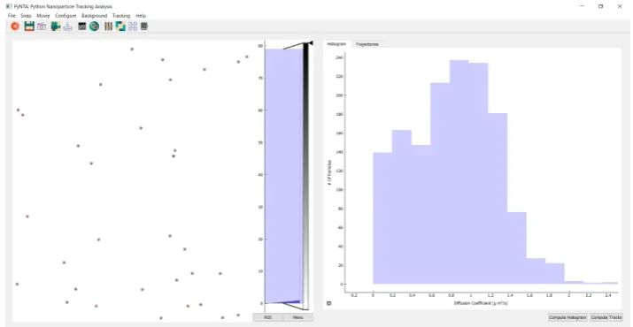
Figure 1.Screenshot of PyNTA. On the left panel, it is possible to observe a frame during the acquisition of a movie. The right panel shows a histogram of diffusion coefficients generated in real-time. The program was developed not only to be efficient but also user-friendly, for example by providing intuitive icons and drop-down menus in the user interface.
frame. The right panel shows the measured distribution of diffusion coefficients. On top of the screen, there is a toolbar which provides quick access to the most common actions, such as starting a free run recording, snapping a frame, setting the region of interest of the camera, etc. The program also includes a configuration window in which the user has a high degree of control over the acquisition parameters such as exposure time, binning, acquisition frame-rate, etc.
Nanoparticle tracking experiments require a set of steps to properly configure various parameters. A common workflow would be, for example: the user snaps a photo, and based on the observation, she would modify the camera settings such as exposure time and intensity threshold. Once satisfied, it is possible to adapt the parameters of the localisation algorithm in order to identify the particles on the image, with instant feedback either on the live feed or on a still image. Detected particles are identified with a red cross on them.
Once the user finds the optimum parameters for localisation accuracy, i.e. an acceptable number of false-positives/negatives, she can proceed to link the extracted coordinates of the particles in each frame to reconstruct the trajectories of single-particles. This step is necessary in order to measure the diffusion coefficient in real time, but it is not mandatory for a successful experiment. Linking and extra analysis steps can be performed a-posteriori on saved data. It is important to point out that PyNTA allows to stream to disk either the raw images, the analysed localisation coordinates, or both. The latter has the advantage of being substantially smaller in size, allowing to stream data much faster. This effectively allows to either increase the duration of acquisition or to work at much higher acquisition frame-rates.
3.2. The Model-View-Controller Pattern
PyNTA was developed following the Model-View-Controller (MVC) structure. This means that the code is separated into different modules, each one in a different folder, and with a clear separation of tasks. These modules are summarised in Fig.2and can be explained as follows:
• Controller: The drivers for the hardware. These modules handle the low-level communication with the devices.
• Model: Specifies the logic and the order of operations to perform a certain measurement • View: User-facing elements, such as the graphical user interface (GUI), or the command-line
Figure 2.Scheme of the Model-View-Controller for laboratory software.Controllersare the drivers for hardware,Modelsimplement the specific steps on how devices are used or the experiment is performed, and theViewis where the user interface is defined.
To further understand the architecture of the code, we specify some of the main contents of each module.Controllerscan be regarded as the drivers for devices, or the Python wrappers for these drivers. Manufacturers of hardware sometimes offer the drivers, such as PyPylon [6] for Basler cameras or NIDAQmx [7] for National Instruments cards. Often, drivers are developed by other researchers, such as the driver for Hamamatsu cameras provided bystorm-control[13]. Sometimes there is no available driver for the cameras and the user will need to develop their own.
Modelsare responsible for defining the logic behind the experiment. A simple case would be an experiment in which it is needed to open a shutter, acquire a frame, close the shutter and save the data. The measurement steps are determined by the user and thus should be separated from the controllers. In Python, this is manifested as different methods for a class calledexperiment. PyNTA specifies steps such asstart_free_run, which starts a continuous acquisition from a camera, orsave_streamwhich continuously saves the acquired images to the hard drive.
Models do not only specify the overall logic of the experiment, they also specify how devices are used. For example, if the camera is set to acquire one frame, to capture a movie one needs to run a sequence of single-frame acquisitions. The advantage of developing models for devices is that they offer common entry points to the user, regardless of the underlying hardware.
We illustrate this point with an example. A camera with a frame-grabber is able to generate movies by acquiring several frames and storing them into a buffer. The computer needs to periodically download the information from the buffer, freeing it for new frames. A camera without a frame-grabber needs to be continuously read out. This two devices work in very different ways, but it is possible to define two models, each with a method calledacquire_moviethat generates the same output: a sequence of images.
The benefits of implementing models for devices may not seem obvious at the beginning, but they become apparent for larger or long-term projects. A common case found in many labs is the need for exchanging the hardware. If the user upgrades or replaces part of the equipment, it is only needed to develop a new model, and the rest of the code will continue to run, including the data acquisition, post-processing, analysis, etc.
real-time plots are built on PyQtGraph [12], a library that gives access to a powerful set of tools for embedding plots in user interfaces. The icons used in the GUI are designed by The Artificial1and released under a CC-BY license.
The view is one of the most challenging aspects of any program, since it requires a different set of skills compared to the rest of the program. Building the view on top of a well-defined model makes it also independent from it. By completely separating the logic of the experiment and the devices from the view itself, it is possible to quickly prototype solutions that in most cases are enough for a researcher.
PyNTA was built strictly following the MVC pattern. This is reflected by the three folders that can be found in the source code, called preciselymodel,view, andcontroller. It has to be noted that PyNTA aims not only at acquiring data, but also to perform a real-time analysis of it. This analysis has a high computational cost, required the program to leverage the possibilities of multi-core processors.
3.3. Distributed Architecture
One common requirement for instrumentation software is to remain flexible over time. A common situation is, for example, a user is monitoring a signal and when everything is ready, she decides to start saving the data, without interrupting the flow. Moreover, she can decide to switch-on a special post-processing task and save the output of it, or just visualise it in real-time. The previous description means that the same information can be consumed by different tasks which may become active at different moments in time. This requirement is not trivial, especially when taking into account that different tasks will be running as different processes without access to shared memory.
Figure 3.Scheme of the underlying architecture that enables the use of multiple processes. A central publisher broadcasts the information to any listening subscriber. Colours depict whether processes generate new data or only consume it. Processes can be started in any order and are completely independent from each other.
In order to develop a flexible, multiprocessing-safe solution, we have developed a specific architecture for themodels. A schematic representation of this architecture can be seen in figure3. One central process, calledpublisher, is in charge of broadcasting the available data to any other processes which are listening to specific topics. For example, the process in charge of acquiring images sends each one of them to the publisher. The localisation process consumes the frames and sends the location coordinates back to the publisher. In turn, the linking process uses this information to build trajectories of the particles. These process have a different colour in the figure because they not only consume the available data but they also generate new information.
There are also dedicated processes for saving the available data, either the images, coordinates of located particles, or linked trajectories. These processes where depicted in a different colour in Fig.3because theyonlyconsume information but do not send anything new to the publisher. This is also the case for the process in charge of calculating the size distribution of the particles based on the trajectories. It has to be stressed that all this exchange of information happens asynchronously. This
means that the process for localising the particles is not waiting for the linking process to finish in order to analyse a new frame.
Not all processes are active at all time, and activation of one specific process does not guarantees that others are also executed. For example, when the camera is acquiring data it is possible to run a separate process to save the images to the hard drive, but it is not required. It is also possible to run a localisation algorithm on each frame, but again, this is not required. These two processes are independent from each other and is the user who decides whether to run them or not. The user can trigger processes whenever she judges that it is useful to store or to analyse the data.
To achieve this degree of flexibility at run-time, we have decided to combine the multiprocessing library of Python with the distributed messaging library ZMQ through its Python bindings called pyZMQ [8]. This combination allowed us to build a Publisher/Subscriber pattern with a very small overhead. Subscribers are the processes discussed in the previous paragraphs and depicted in Fig.3. Each subscriber is a separated python process, thus leveraging the multi-core capabilities of modern computers. The computational cost in this approach comes from the need to serialise/deserialise python objects in order to transmit them from one process to the other, but it has an overall small impact.
ZMQ is a library which relies on sockets to exchange information. The main advantage of relying on sockets is that they are available in mostly, if not all, programming languages. Therefore, the information generated by PyNTA can be easily consumed by any other program, written in any other language, which is able to listen on a specific port. This feature makes the program very easy to extend by developers with different knowledge-sets. Moreover, this architecture opens the door to distributed solutions, exchanging information not only on the same computer but over the network.
3.4. Tracking Particles and Linking Trajectories
The tracking and linking algorithm for the localisation of nanoparticles are based on the excellent Trackpy library [5,9], which implements the Crocker and Grier algorithm [4] in Python. Data is saved in HDF5 format, which makes it compatible with most data analysis programs and workflows. It is also possible to convert the data into plain ascii files with simple tools available online.
The design of the program makes it simple to replace the algorithms in case there is a better solution for a ceratain user’s needs. Within the model module, the localisation subroutines expose the workflow for identifying and linking trajectories.
3.5. Performance Testing
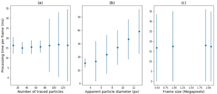
To check program dependencies and evaluate the performance of different PyNTA methods, an iPython notebook has been provided with the package,examples/test_tracking_speed.ipynb. The design of Pynta allows it to run without a GUI, therefore this notebook can also be used as a reference for testing the installation and time performance of the different tracking steps. This part can also be tested without connection with the hardware and based on simulated data, using the module namedSimBrownian, which also gains access to "ground data" for possible tests of other tracking algorithms. This module also provides the possibility of accumulating frames into memory in order to loop through them instead of keep simulating data. We tested the dependence of the average analysis time per frame on frame size, apparent particle diameter, and number of particles in the frame, by running this notebook on a laptop with an Intel i7 processor. Dependence of the average processing speed per frame on three most plausible measurement parameters are tested based on simulations and results are presented in Fig.4. Among the tested parameter, the apparent particle size has the biggest influence on slowing down the analysis process.
3.6. Addition and customisation
Figure 4. . The average processing speed per frame for various measurement conditions. (a) dependence on the number of particles present in each frame with apparent particle diameter of 3 pixels, (b) dependence on the apparent particle diameter for an average 50 particles in each frame, and (c) dependence on the frame size, for apparent particle diameter of 3 pixels and 50 particles in each frame.
inquire what parts of the code to alter in order to meet their needs. This flexibility is best explained through an example. A foreseeable desired feature could be to track complex objects, such as cells, animals, etc. Any algorithm that allows to extract coordinates of objects out of an image can be easily integrated following the documentation and the existing code as an example.
Consider the case of a developer who wishes to add support for choosing the region of interest (ROI) in the image before acquiring data from the camera. Assuming that the driver for the camera supports such a feature, the user should search in themodelfolder and find a sub-folder calledcameras. In that folder, there is a python file with the brand of the camera.
In the model for the camera, the developer will find a collection of methods such assetExposure
ortriggerCamera. Next to those methods, she can develop a new one called, for example,setROIthat
takes as arguments the coordinates of the corners of the region of interest. Then, she will proceed to develop the steps needed to set the region of interest in the camera using the controller’s methods.
The next step is to develop a method that can handle the ROI in the experiment model, which can be found inside theexperimentsfolder within the model folder. This method will handle the input of the new coordinates, will pass it to the camera model and will update the necessary parameters, such as buffers, to the new image size.
The final necessary action is to update the view in order to handle the ROI input. This can be achieved by developing a widget in which the user can input the coordinates, or the main window widget can be expanded to allow some mouse interaction. In any case, the view will grab these values and will use the method available in the experiment to update the ROI.
This example is actually implemented in the code and can be used as a reference for developers who would like to expand the code. It is relatively straightforward to follow the different connections between different parts of the code if one follows the steps just described.
4. Discussion
The code is under git version control and hosted on Github. This means that any user interested in improving or fixing issues can fork the code onto their own repository. The changes can then be submitted as a pull request with appropriate descriptions. After reviewing the code, accepting the changes is straightforward. This procedure is very transparent and allows to give proper credit to different contributors.
Current processing speed of the software is mainly limited by the rate at which frames can be analysed. In order to investigate the limitations of the program, we performed the tracking on simulated data, in which the particle behaviour is well defined. The computational cost of the Crocker and Grier algorithm depends on different factors such as the frame size but also on the particle diameter. During our tests, identifying 50 particles with an average diameter on the camera of 5 pixels takes approximately 17mson a dedicated core of an Intel i7 processor. 60 frames per second on a 12−bit, 2Mpixcamera amounts to roughly 170MB/sof data. On the other hand, the localisation of 50 particles at the same frame rate amounts to roughly 60kB/s, three orders of magnitude lower than for recording the full frame.
The linking procedure, i.e. identifying locations in different frames as belonging to the same particle, implements a maximum likelihood algorithm. The algorithm speed also depends on different parameters, such as the number of particles on a frame and the maximum estimate distance for the movement of a particle between two successive frames. In the cases studied in which between 10 and 50 particles were present on each frame, the linking algorithm proved to be faster than the identification algorithm. However, further tests need to be carried on to identify its limitations.
5. Conclusions
Nanoparticle tracking analysis is a tool that is gaining momentum in different fields. We believe that a timely tool such as PyNTA can enhance the development of the technique. By building the program using Python, we give access to a broad community of researchers in different fields to further enhance the tool in a collaborative way.
With PyNTA, researchers can easily perform experiments on existing setups, lowering the overhead that implies the acquisition of new hardware. Any wide-field microscope is readily available to perform nanoparticle tracking experiments. Leveraging the capabilities of live particle tracking, PyNTA reduces the amount of data that requires saving, which translates to the possibility of increasing the acquisition frame rate and duration. Moreover, the capability of estimating the size distributions while the acquisition is running, allows researchers to preform on-spot adaptive experiments.
6. Availability of software
The PyNTA package currently provides interfaces for Hamamatsu, Photonic Science, and Basler cameras. The code is available on Github2, together with its extensive documentation both for users and future contributors3.
Author Contributions: Conceptualisation, A.C. and S.F.; methodology, A.C. and S.F..; software, A.C.; validation, A.C. and S.F.; formal analysis, A.C. and S.F.; investigation, A.C. and S.F.; resources, A.C. and S.F. and A.P.M.; data curation, A.C.; writing original draft preparation, A.C. and S.F.; writing, overview and editing, A.C. and S.F. and A.P.M.; visualisation, A.C.; supervision, S.F. and A.P.M.; project administration, S.F.; funding acquisition, S.F. and A.P.M.
Funding:This research was supported by the Dutch Organisation for Scientific Research (NWO)
Acknowledgments: PyNTA is built on open source tools developed by researchers, such as Trackpy [9] and Pyqtgraph [12], and draw inspiration from packages such as storm-control [13], Instrumental [11], and Lantz [10]. Moreover, it wouldn’t have been possible without a much broader community that built libraries like ZMQ, Qt, and Python.
Conflicts of Interest:The authors declare no conflict of interest.
Abbreviations
The following abbreviations are used in this manuscript: NTA Nanoparticle Tracking Analysis
MSD Mean Square Displacement MVC Model-View-Controller
References
1. Chenouard, N.; Smal, I.; de Chaumont, F.; Maska, M.; Sbalzarini, I. F.; Gong, Y.; Cardinale, J.; Carthel, C.; Coraluppi, S.; Winter, M.; et al. Objective Comparison of Particle Tracking Methods. Nature Methods2014,
11, 281-289, https://doi.org/10.1038/nmeth.2808.
2. Faez, S.; Lahini, Y.; Weidlich, S.; Garmann, R. F.; Wondraczek, K.; Zeisberger, M.; Schmidt, M. A.; Orrit, M.; Manoharan, V. N. Fast, Label-Free Tracking of Single Viruses and Weakly Scattering Nanoparticles in a Nanofluidic Optical Fiber. ACS Nano2015,9 (12), 12349?12357. https://doi.org/10.1021/acsnano.5b05646. 3. Hassan, P. A.; Rana, S.; Verma, G. Making Sense of Brownian Motion: Colloid Characterization by Dynamic
Light Scattering. Langmuir2015,31, 3?12. https://doi.org/10.1021/la501789z.
4. Crocker, J. C.; Grier, D. G. Methods of Digital Video Microscopy for Colloidal Studies. Journal of Colloid and Interface Science1996,179, 298?310. https://doi.org/10.1006/jcis.1996.0217.
5. Allan, D. B.; Caswell, T.; Keim, N. C.; van der Wel, C. M. Trackpy: Trackpy v0.4.1; Zenodo, 2018. https://doi.org/10.5281/zenodo.1226458.
6. The official python wrapper for the pylon Camera Software Suite, Available Online: https://github.com/basler/pypylon (Accessed on 17 June 2019).
7. A Python API for interacting with NI-DAQmx, Available Online: https://github.com/ni/nidaqmx-python/ (Accessed on 17 June 2019).
8. PyZMQ: Python bindings for zeromq, Available Online: https://github.com/zeromq/pyzmq/ (Accessed on 17 June 2019).
9. Python particle tracking toolkit, Available Online: github.com/soft-matter/trackpy (Accessed on 17 June 2019).
10. Lantz: Simple yet powerful instrumentation in Python, Available Online: https://github.com/lantzproject/lantz (Accessed on 17 June 2019).
11. Python-based instrumentation library from the Mabuchi Lab, Available Online: https://github.com/mabuchilab/Instrumental (Accessed on 17 June 2019).
12. Scientific Graphics and GUI Library for Python, Available Online: http://www.pyqtgraph.org/ (Accessed on 17 June 2019).