An Intuitive and Realistic Visualization Method for Seabed Terrain

An Intuitive and Realistic Visualization Method for

Seabed Terrain

Zixian Xiao1,2,†, Liheng Tan2,†,*, Xiong You3,, Hongli Liu3,and Bingchuan Jiang4,

1 _{State Key Laboratory of Geo-Information Engineering, Xian 710000, China; vrlab [email protected] (Z.X.);}

2 _{Information Engineering University, Zhengzhou 450000, China; vrlab [email protected] (L.T.);}

[email protected] (X.Y.); [email protected] (B.J.);

3 _{Communication University of China, Beijing 100020, China; [email protected] (H.L.);}

* Correspondence: vrlab [email protected]

† These authors contributed equally to this work.

Abstract: Visualization of the seabed terrain is one of the key functions of marine geographic information systems. The major challenge arises from the fact that the obtained data for seabed terrain usually consists of elevation and sediment only but does not include remote sensing images, which is crucial for ground terrain visualization, as they can be used as textures to reveal detailed information and achieve realistic visual results. Existing seabed terrain visualizing methods (including annotations, color-mapping, and texture-mapping) have limitations in reality and intuition, as they are inadequate to express the physical characteristics of sediments accurately. This paper presents a novel and advanced 3D visualization methods of seabed terrain, through which the physically based rendering theory is introduced into the field of geographic visualization. We analyze the main categories of seabed sediments as well as their optical features, then develop a procedural method to generate physically based rendering materials for different sediments. Next, a state-of-the-art bidirectional reflectance distribution function is adopted to achieve accurate and intuitive terrain rendering. We also refine the texture sampling method and propose a strategic seabed objects generation method to establish a more natural and realistic undersea ecologic terrain. Experimental results revealed that our method can make good use of the limited seabed terrain data and get significant improvements in visual effect, which could enable users to perceive and analyze the seabed geographic environment more accurately and intuitively.

Keywords:Seabed; Sediment; Terrain; Visualization; Physically Based Rendering; Realistic

1. Introduction

The research items of marine surveying and mapping comprise of the ocean, rivers, lakes, and surrounding lands, which account for 71% of the earth’s surface. Geometry, physical, humane, and other geography-related properties of the marine environment are of primary concern.

They’ve immensely contributed to the acquisition, processing, management, or visualization of ocean environment data [1–3]mostly owing to the tremendous amount of studies made. Among them, visualization of seabed terrain is obviously one of the most important research topics of the marine geographic information system (MGIS). An accurate, scientific, and intuitive terrain visualizing approach significantly benefits the cognition of marine geographic environment. Moreover, seabed terrain visualization also provides a primary geographic reference, which is the essential prerequisite for most other applications in the MGIS, such as underwater positioning and navigation, visualization and analysis of other kinds of ocean environmental data (e.g. water temperature, salinity and density) and marine meteorological data (e.g. air pressure and humidity).

Visualization of ground terrain has been well discussed in the traditional surveying and mapping field. Terrain data can be obtained through ground measurements, remote sensing, and photogrammetry. Digital elevation model (DEM) and digital orthophoto map (DOM) are typical forms

of acquired data. It is therefore convenient to firstly construct the geometric shapes of terrain in 3D GIS based on DEM, and then use digital orthophoto maps as textures in order to express detailed information. Considering that the textures can reveal the ground-truth optical characteristics of the terrain surface, this kind of method can achieve accurate and realistic visual results of terrain with highly accurate DEM and DOM data.

However, some challenges appear when it comes to the visualization of seabed terrain since the significant differences from ground terrain in data-wise exist. Seabed terrain data can be typically obtained through a multi-beam depth sonar system, strata plane surface instrument, analytic drilling, or field investigation. The primary forms of output data at the seabed are mostly DEM and sendiment information. It is quite impossible to acquire large-scaled remote-sensing images of seabed terrain, which appears to be due to the light absorption and scattering effects of seawater. The scarcity of orthophoto maps will significantly reduce the available information and put forward new requirements for visualizing the seabed terrain, compared to the ground terrain. So we incline to explore every possible usage of the limited seabed data, which aims to strengthen the expression of geometric features of DEM. We also aim to discover new means to model and reveal the optical characteristics and effects of seabed sediments since the lack of actual seabed images. An accurate, intuitive, and realistic virtual seabed terrain environment can be constructed in this way, which helps users to better cognize the information contained in seabed surveying and mapping data [4,5].

Existing associated studies from the geo-information field usually attain three-dimensional seabed terrain visualization by making use of simple illumination models (e.g. hill shading), annotations, and feature textures. Although these methods distinguish regions of different sediments effectively, they have some shortages as well. The results fail to represent the sediment features well and lack a sense of reality and intuition in several cases, as the modeling and visualizing processes are not designed well enough according to the physical and optical properties of the different sediment surfaces.

In this study, a real-time data-driven seabed terrain visualization method is proposed by implementing the physically based rendering (PBR) theory and several advanced texturing techniques. The proposed method structures and visualizes different seabed sediments in a more physical way, and thus significantly improves the accuracy and intuitiveness of the visualization effects of seabed terrain. This paper’s key contributions are summarized as follows:

• Physically-based rendering methods are applied to the visualization of seabed terrain, which inturn promotes the sense of reality.

• Optical characteristics of numerous types of seabed sediments are analyzed and associated rendering models are designed to synthesize the rendering effects.

• A method for blending different sediment surfaces in accordance with the accumulated thickness is designed, which preserves details of different layers and also enables flexibility for the perceptual effect.

• Detailed and realistic seabed textures are generated stochastically with the help of a couple of texture patterns, which is conducive to realize realistic visualization of seabed terrain.

2. Related Works

Compared to ground terrain data, obtaining seabed terrain data has a higher cost and can only get fewer data-type. Under-water photogrammetry is inefficient, and the digital orthophoto map is nearly impossible to get. The major challenge of seabed visualization is to produce an intuitive and accurate result with limited survey data. The target of visualization includes elevation and sediment distribution, but the elevation is the research hot spot of seabed visualization in the early days due to the restriction and inconvenience related to obtaining sediment data.

contour. Different from the notation method that directly uses raw data, this method processed and then draw imaginary contours to represent the variation trend of seabed depth. Lin et al. [6] managed to combine this method and color-mapping methods to simulate the lighting effect on seabed terrain inorder to get a stereoscopic image. (3) Color-mapping. This method maps colors to the depth of seabed, thus creating a sense of depth. Ma et al. [7] replaced the widely used RGB color model with the HSL color model, from which both height detail and terrain feature are revealed through the illumination of the mapped color. (4) Hill-shading. As the most realistic visualization method, hill-shading initially creates a virtual parallel light source and then calculates every pixel illumination found on the map determined by the angle between light direction and terrain slope. Wei et al. [8] discussed the method of generating 2D and 3D shaded relief maps from raw depth data. In their discussion, both interpolation and rasterization are used as methods to generate TIN (triangular irregular network) and DEM (digital elevation model),nonetheless, the illuminating effect is adjusted to get better hill-shading results.

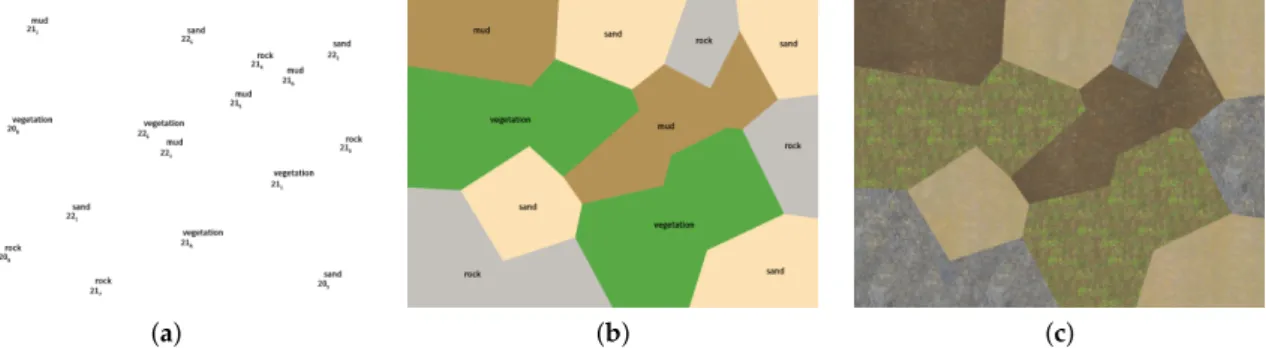
With the invention and development of high-precise marine survey and mapping devices (e.g. side-scan-sonar and sub-bottom profiler), the precision of seabed elevation data promoted and detailed sediment distributions are available for people to obtain and analyze. In this case scenario, sediment visualization becomes a topic in the field of marine GIS. The mainly used visualization methods of seabed elevation can be listed as follows: (1) Annotation. (SeeFigure1(a)) Same as depth annotation method in elevation visualization, this method also marks the sediment characteristic to certain points coordinates. Many electronic chart systems (ECS) have been using this method in the early days to mark the sediment distribution. (2) Color-mapping. (SeeFigure1(b)) Similar to the mentioned method above, this method uses different colors to represent different sediments. Liu et al. [9] managed to construct a multi-layer sediment distribution model using color-mapping and interpolation based on the water depth data and multi-beam data. (3) Texture-mapping. (SeeFigure1(c)) Different from color-mapping, texture-mapping uses texture patterns to represent different sediments. Zhang et al. [10] introduced a simple way to distinguish different sediments by using parallel lines with various angles as sediments’ texture pattern. Chen et al. [11,12] captured the real world’s sediment image and used the image samples as textures to represent different sediment in the visualization result. Besides, they implemented texture transition zones with the equidistant line to realize the smooth transition between sediments [11,12], but the blending result of this method is still quite different from the actual seabed environment. The blending method [13] proposed by Andrey M. solved this problem by combining height maps and weights, which could get a transition zone with more texture details.

(a) (b) (c)

Figure 1. Different sediments visualization methods. (a) Annotation method. (b) Color-mapping method. (c) Texture-mapping method.

by using the texture sample from the real world despite the fact that sometimes it’s hard to tell the difference between textures.

As far as elevation visualization is concerned, depth notations use the most accurate raw data. However, the variation trend of seabed depth is unclear. Depth contour visualizes the basic shape and variation trends of seabed terrain using contour lines, but it loses the detail of depth variation if the contour intervals are not suitable. Color-mapping maintains the most detailed seabed elevation but it’s hard to read the accurate depth using the color map. Hill-shading has the most realistic and intuitive visualization result, but it is nearly impossible for users to read the actual height of seabed terrain directly from the map.

After consideiring the above methods’ pros and cons, we can simply conclude that elevation visualization is pursuing a stronger three-dimensional sense while sediment visualization is aiming at improving intuition. In this case, we introduce the physically based rendering (PBR) theory [14] into the field of geographic visualization to model and visualize the seabed terrain. The proposed method can not only visualize the elevation information and diffuse reflection of seabed sediments but also simulate and represent the sediments-related optical phenomenon including specular reflection and environment lighting. With information adding to the scene, the sediment texture became more realistic hence rendering the result more intuitive compared to the methods discussed earlier. Besides, we improved our texture blending and sampling method to make our results more natural and more detailed.

3. Our Methods

3.1. Analysis and Processing of Typical Seabed Topography Data

Surfaces in the marine geographical environment can be divided into organic and inorganic surfaces. There’s a vast area occupied by vegetation (e.g. aquatic plants and coral) with organic surfaces coverage. The inorganic surfaces can be further subdivided into rocky surfaces, muddy surfaces, and sandy surfaces with respect to the inorganic particles’ size and surface characteristics. In the present study, seabed data are collected and processed originally to visualize the distribution of these surfaces.

During seabed data acquisition, altitude data of seabed can be collected from satellite images or acoustic detection [15]. The precision range of satellite-based remote sensing method is about 10-100m. Even though capturing images from satellites have a high measurement speed, it is only applicable to coastal waters. Similar to satellite mapping, airborne mapping has a precision range of about 1-1000m, and its measurement speed is lower than that based on satellite. However, the measurement depth can reach as high as 6m. The precision of the side-scan sonar radar is raised to 0.01m. Moreover, the measurement depth of this kind of device can reach hundreds and even thousands of meters, which is attributed to no media changes (from air to seawater) and interferences of the aircraft’s instability. The X-ray surveying and mapping methods have the highest precision (0.001m) amongst all these methods, but its measurement speed is relatively low. [16] Appropriate surveying and mapping methods can be chosen according to practical demands in different scenes to collect sediment data and altitude data with the required different precisions. Additionally, the reflectance of echo’s reflection, cumulative energy normalization curve, time-domain waveform features of reflected signals (e.g. statistics and histogram on amplitude distribution), frequency domain features of reflected signals and inter-Ping relevant statistical information can be collected by acoustic detection devices to make further analysis. Assisted with drilling sampling at key points, it is able to acquire more accurate information about both sediments and altitude.

Using the modified classification models of Shepard and Folk [17–19], sediments consisting of different clastic components can be classified into several categories depending on the ratio of mud (particle size less than 63 µm), sand (particle size between 63 µm and 2000 µm) and gravel (particle size greater than 2000 µm). To simplify the presentation for subsequent steps, we implemented a simplified classification model by using a hierarchical model of "rock-mud-sand-superficial vegetation" from the bottom to the top (SeeFigure3).

Figure 2.The data structure used in this study. We store the height information in a 32-bit bitmap and layers’ thickness information in the RGB channels of a 24-bit bitmap.

(a) (b)

Figure 3.(a) Modified Folk’s [20] classification method. (b) Our simplified classification method for inorganic sediment. Organic sediments are absent in this model and considered separately.

177 Seeing that the process of data acquisition and processing is out of scope, we use the existing 64m2topographic data with a 1m precision scale in this study. (SeeFigure5)

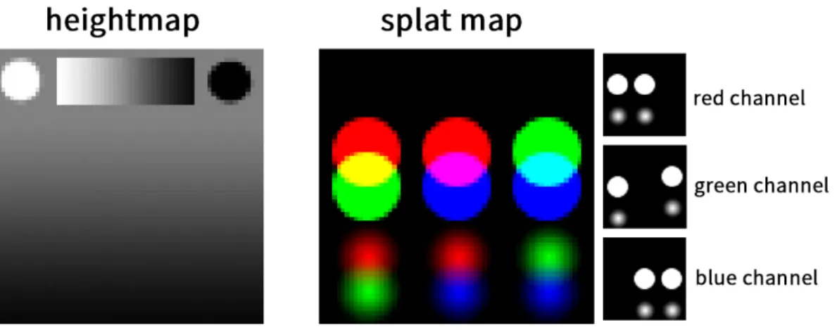
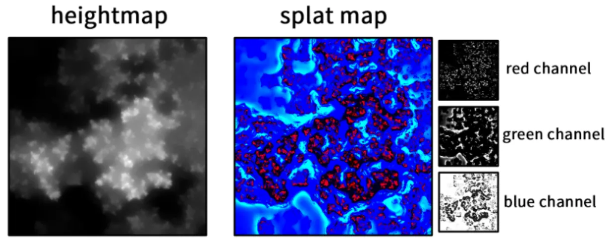
Figure 4.Decomposition of different layers and information maps. The overall shape of the seabed terrain is depicted by the heightmap, while the thickness maps contribute to the appearance of sediment surfaces and fine details.

Figure 5. The adopted data structure in this study comprises of a heightmap and a splat map. The heightmap stores 32-bit floating-point height values of the seabed terrain and the splat map stores 8-bit thickness values in the three channels of the splat map.

3.2. Physically-Based Illumination Model (PBR Model)

For comprehensive consideration of performance and effect, The Torrance-Sparrow BRDF (bidirectional reflectance distribution function) [21,22] illumination model is applied. This model has been verified and deemed valid by ray-tracing renderers [22–24]. Furthermore, this model has a high efficiency [25–27]. The BRDF model is defined as:

fr(wo,wi) = kd

π + ks 4π(n·wi)

·D(h)·F(wo)·G(wo,wi) (1)

Terms in this formula are introduced as follows:

• kdandksare the albedoes of diffuse and specular reflection, wherekd+ks ≤1.

• TheDterm gives a distribution of the normal arrangement of the microfacets that are aligned relative to vectorh. We use the GGX distribution function [28].

• Fterm gives the physical reflection ratio of incident lights. Here, Schlick approximation [29] is applied for the sake of operational efficiency.

• Gterm uses the Smith Joint Masking-Shadowing Function [30] which is characteristic of high efficiency and good visualization effect.

Direct illumination with the ideal light source (e.g. the sun) is easy to be achieved in the BRDF model. The rendering effect can be gained only by calculating the illumination energy and inquiring shadow maps.

For diffuse reflection, indirect illumination, [31] proposed a method to store indirect environmental illumination energy by using the spherical harmonics. The spherical harmonics lighting probes array is calculated in terrain regions and the indirect Lambert reflection is computed by sampling the probes and finally refined by Screen Space Ambient Occlusion (SSAO) [32]. Specular indirect illumination effects are calculated by combining Screen Space Reflection (SSR) and reflection probes with references to [33].

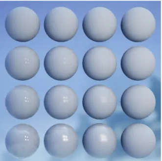
A realistic renderer is built based on the above method. This renderer can calculate real visual effects according to albedos, indices of reflection, roughnesses, and normals of the surfaces.Figure6

reveals the render result using the above method. We interpolated different parameters (indices of reflection and roughness) to examine the perceptual effect.

Figure 6.Rendering of materials with different parameters. Note that the roughnesses increase from left to right and the indices of reflection increase from top to the bottom.

3.3. Sediment Texture Seeds

Photogrammetry is widely used in the multi-media industry [34,35]. Realistic rendering requires a lot of information about the surfaces to be rendered, which is generally stored in textures and is difficult to obtain. A common method to synthesize such information is photogrammetry. Photos with proper white balance are captured firstly, and then point clouds are reconstructed in accordance with the photos. The required information can be obtained through the constructed point cloud data.

reference to [36] to get a balanced luminance, then blend the textures as discussed as follows, and finally synthesize the output via the adopted illumination model.

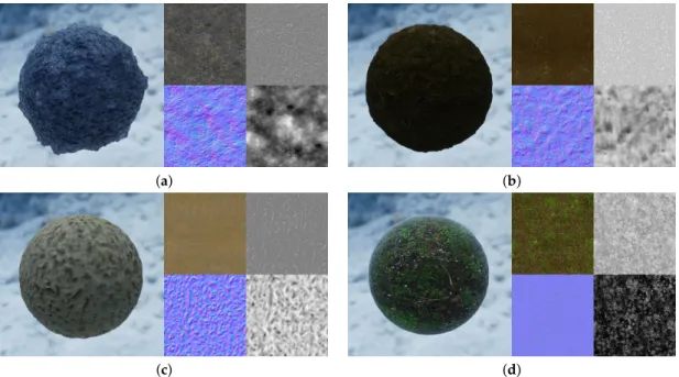
SeeFigure7for the photogrammetry texture assets in this study.

(a) (b)

(c) (d)

Figure 7.Different sediment texture seeds produced using photogrammetry. (a) Rock sediment. (b) Mud sediment. (c) Sand sediment. (d) Superficial vegetation sediment. The photogrammetry process provides albedos, roughnesses, normals, and bumps, which are vital in the adopted visualization method.

3.4. Materials Blending

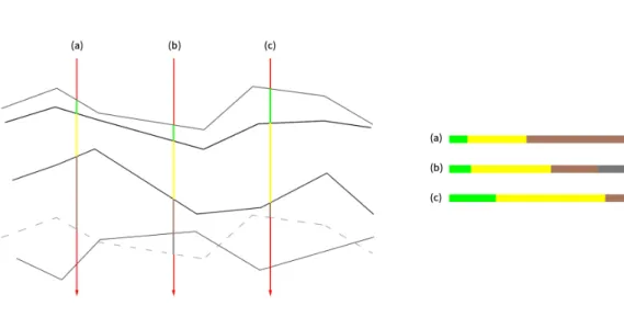
In this study, the terrain shape is expressed as units of uniform quad meshes. Different weight layers are stored in the multi-channel splat maps. We accumulate the thicknesses from the top of the seabed to the lower sediments. The algorithm is illustrated inFigure8and can be described as follows:

1. Initialize the cumulative thickness to 0.

2. Inquire thickness of sediments at the current layer and judge whether its thickness and the cumulative thickness exceed the threshold. If yes, turn to Step 4.

3. The blend ratio in the current layer is used as the thickness of the layer. This thickness is summed to the cumulative thickness. Then, turn to sediments at the next layer and return to Step 2. 4. The material ratio in the current layer is equal to (threshold-cumulative thickness).

Figure 8.Calculate the blend ratios from thickness information. Different colors represent the blend ratio of the corresponding layers.

Since we use a four-layer sediment model, the algorithm can be expanded intoAlgorithm1. The input thickness information of 4 layers is stored in the static splat map, but these sediments’ output ratio is dynamic and can be adjusted by updating the threshold of accumulated thickness.

Algorithm 1Calculate blend ratios

1: procedureCALCULATE THE BLEND RATIOS FOR THE THE4LAYERS 2: a←Thickness of superficial vegetation layer

3: b←Thickness of sand Layer 4: c←Thickness of mud layer

5: t←Threshold of accumulated thickness 6: ifa + b >= tthen

7: ratio←vec4(a,t−a, 0, 0) 8: else ifa + b + c >= tthen 9: ratio←vec4(a,b,t−a−b, 0) 10: else

11: ratio←vec4(a,b,c,t−a−b−c) 12: returnratio

A height-based blending method proposed by Mishkinis [13] is applied for extension during material blending. The blending effect is refined according to the smoothing factor of different layers. The algorithm can be found inAlgorithm2.

In the Mutate procedure, we sample the bump value from texture A and B at the specified coordinates as the local thickness mutation and combine it with the thickness information. Then, we calculate these two layers’ blending weight. The sharpness of the transition between different sediment layers is influenced by the Smoothness parameter in this procedure (SeeFigure9).

(a) (b) (c) (d) Figure 9. (a)The splat map.(b),(c),(d)Blending effect of increasing blending hardness. Algorithm 2Layer Blend

1: procedureMUTATE

2: BumpA ←Sample from A

3: BumpB←Sample from B

4: ratio←Initially computed blend ratio of texture B 5: Smooth←Smoothness of transition

6: αA←(1−ratio)∗BumpA

7: αB←ratio∗BumpB

8: delta←αA−αB

9: returnsmoothstep(Smooth,−Smooth,delta)

10: procedureCALCULATE THE FINAL SEDIMENTATTRIBUTION 11: αVS←Mutate(HVegetation,HSand,ratioratio.x+ratio.y .y,Smooth)

12: αVSM←Mutate(max(HVegetation,HSand),HMud,ratio.x+ratioratio..zy+ratio.z,Smooth)

13: αVSMR←Mutate(max(HVegetation,HSand,HMud),HRock,ratio.x+ratioratio.y+ratio.w .z+ratio.w,Smooth)

14: AttrVS ←lerp(AttrVegetation,AttrSand,αVS)

15: AttrVSM←lerp(AttrVS,AttrMud,αVSM)

16: AttrVSMR←lerp(AttrVSM,AttrSand,αVSMR)

17: returnAttrVSMR

3.5. Visual Effect Enhancement

3.5.1. Tri-Planar Mapping

(a) (b)

Figure 10.(a) Textures are projected using terrain’s UV coordinates. (b) Textures are projected using tri-planar mapping.

3.5.2. Anti-Tiling

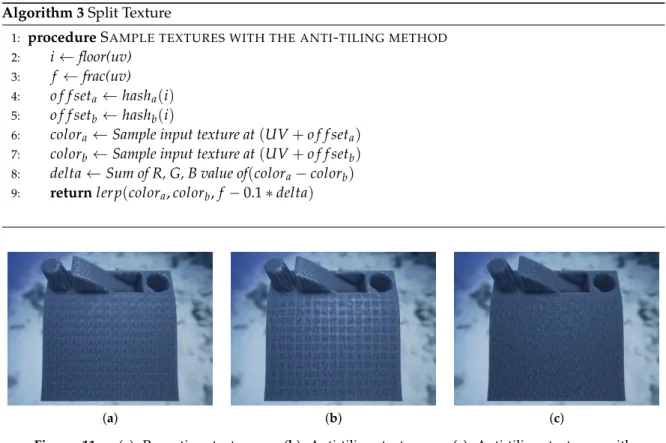
Limited by the storage space, it is hard to cover the whole terrain without repeating the textures. However, realism may be severely affected by the repetition of textures which will produce artifacts. It is necessary to 249 reduce the artifact to assure the randomness and ascertain the nature of the seabed terrain’s texture. A tiled texture can be extended by implementing Quilez’s [38] method. The detailed algorithm can be found inAlgorithm3. SeeFigure11(a)(b)for how this procedure improves the visual effect.

Algorithm 3Split Texture

1: procedureSAMPLE TEXTURES WITH THE ANTI-TILING METHOD 2: i←floor(uv)

3: f ←frac(uv) 4: o f f seta←hasha(i)

5: o f f setb ←hashb(i)

6: colora←Sample input texture at(UV+o f f seta)

7: colorb←Sample input texture at(UV+o f f setb)

8: delta←Sum of R, G, B value of(colora−colorb)

9: returnlerp(colora,colorb,f−0.1∗delta)

(a) (b) (c)

Figure 11. (a) Repeating textures. (b) Anti-tiling textures. (c) Anti-tiling textures with histogram-preserving blending operators. Note how the repeating patterns influence the quality of the visual effect.

3.5.3. Histogram Color Preservation

To further reduce the repetition effect and strengthen the sense of reality, pre-processing of textures is implemented using the Heitz’s method [39] to preserve the color distribution. This process undoubtedly improves the visual effect. The histograms of the textures are preserved so that the brightness and color are well balanced to eliminate any blend seams. (SeeFigure11(c)).

3.5.4. Aquatic Plants Generation and Blending

It is necessary to add sediment details to confirm the authenticity of the visual effect. In this study, the coral reef model, seagrass model, and rock model are used as surface features. Surface features are generated procedurally based on the blend ratios of different sediments.

The position of the surface features is controlled by the divide-and-conquer method. The terrain is divided according to the horizontal and vertical coordinates into several blocks with fixed size. Each block uses an ID as the seed of pseudo-random sequence to generate a random stream. Corresponding surface features are generated at the coordinates produced by the random stream based on the proportion of sediments. (Figure12)

(a) (b)

Figure 12.(a) Without surface features. (b) With surface feature. Note how surface features enhance the visual richness and correctly reflect the seabed environment.

(a) (b)

Figure 13.(a) Not blending with the terrain. (b) Blending with the terrain based on the delta height.

3.5.5. Underwater Environment Simulation

To further enrich the photorealism, we apply volumetric rendering [40] to create the basic underwater atmosphere. Later, color temperature and white balance are adjusted to achieve a more realistic simulation of the underwater environment (Figure14).

(a) (b)

Figure 14.(b) is the rendering result after apply volumetric rendering effect and color correction to (a). (b) produces a more realistic seabed environment simulation to the users.

4. Experiment

Figure 15.The texture maps that will be used in the following experiment below.

After the above processes, a uniform quad grid terrain is produced according to the heightmap. Figure16displays the blend effect of the proposed method. Note the jagged edges between the sediment layers inFigure16(a) are due to the limitations of texture resolution. The artifacts are removed inFigure16(b)by implementing the Mutation procedure.

(a) (b)

Figure 16. Visualization of blend effect of the proposed method. (a) Original splat map. (b) Blend result after the Mutation procedure

.

We compare the visual effect of terrain rendered using the Lambertian reflection model and the above-mentioned PBR model discussed previously in (SeeFigure17). The traditional Lambertian Shading results in a lack of indirect illumination and photorealism, which is addressed by the PBR shading model.

(a) (b) (c) (d)

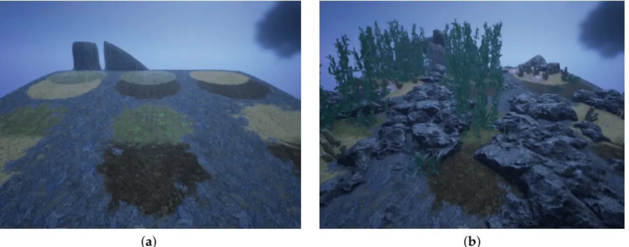
Next, the sediment texture is enhanced by the method discussed in Section3.5.2and3.5.3(See Figure18). Note that the anti-tilling method eliminates repetitive patterns and the tri-planar mapping method reduces texture stretching on the cliff. The method in Section3.5.4is used to generate surface features (SeeFigure19) which further enhances the realism of the seabed terrain.

(a) (b)

(c) (d)

(a) (b)

Figure 19. (b) correctly reflects the surface features of the seabed environment, while (a) does not include surface features and thus fails to achieve the intuitiveness as (b).

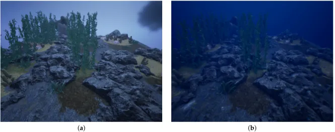
Finally, volumetric rendering and color grading is conducted, which simulates the photorealism for the seabed environments and made the visualization result more realistic. (SeeFigure20)

(a) (b)

Figure 20.Both images are rendered from a fixed point of view. Comparing with (a), (b) introduces volumetric rendering to simulate the underwater visual effect, which greatly enhances the simulation of photorealism.

5. Conclusions

Author Contributions: conceptualization, Z.X. and L.T.; funding acquisition L.T.; methodology, Z.X. and L.T.; project administration L.T.; resources, Z.X. and Y.X. and H.L.; software, Z.X. and H.L.; validation Y.X. and B.J.; writing–original draft preparation, Z.X.; writing–review and editing, Z.X. and L.T. and H.L.;

Funding: This research was funded by State Key Laboratory of Geo-Information Engineering (Grant No. SKLGIE2018-M-4-1) and National Natural Science Foundation of China (Grant No. 41901334 and 41801319).

Conflicts of Interest:The authors declare no conflict of interest.

Abbreviations

The following abbreviations are used in this manuscript:

BRDF Bidirectional Reflectance Distribution Function DEM Digital Elevation Model

DOM Digital Orthophoto Map GIS Geographic Information System MGIS Marine Geographic Information System LUT Look Up Table

PBR Physically Based Rendering SSAO Screen Space Ambient Occlusion UAV Unmanned Aerial Vehicles

References

1. He, L. Research on Key Issues of Sediment Classification for Seabed and Sub-bottom Based on Multi-beam and Sub-bottom Profile Echo Intensity. Journal of Geodesy and Geoinformation Science2016, 45. 2. Jiang, X. Study on the Integration and Fusion Models of Spatial Data Collected by Submarine Sub-bottom

Acoustic Exploration with Its Representation in GIS. Phd. thesis, Faculty of Science, Zhejiang University, 2009.

3. Nie, J.; Chen, H.; Zhang, J.; Guo, D. Interactive integration visualization of multidimensional marine data based on the data similarity degree. Marine Science Bulletin2015, 34, 586–591.

4. Chapman, P.; Wills, D.; Brookes, G.; Stevens, P. Visualizing underwater environments using multifrequency sonar. IEEE Computer Graphics and Applications1999, 19, 61–65. doi:10.1109/38.788801.

5. Su, C.; Yu, W.; Ni, G.; Huang, Z.; Tao, C.; Zhang, X. Display and control system for deep water multi-beam bathymetric side-scan sonar. Journal of Zhejiang University (engineering)2013, 47, 934–943.

6. Ling, Y.; Peng, R. Research on Sea Floor Three-Dimensional Vision Based on Illuminated Depth Contour and Color Gradients. Hydrographic Surveying and Charting2009, 29, 29–31.

7. Ma, D.; Yang, F.; Cui, X.; Tian, H. A Method of Drawing Three-dimensional Submarine Topographical Rendering Map Based on OpenGL. Journal of Shandong University of Science and Technology(Natural Science)2018, 37, 99–106.

8. Wei, J.; Fang, Q.; Qi, Y. Research on Methods of Drawing Three-dimensional Submarine Shaded Relief Map. Hydrographic Surveying and Charting2013, 33, 60–62.

9. Liu, Z.; Jin, J.; Liu, Z.; Weng, Z.; Wei, Z.; Wang, F. The preliminary study to sea base matter three-dimensional visualization simulation. SCIENCE OF SURVEYING AND MAPPING 2008, 33, 113–115.

10. Zhang, L.; Wang, Y.; Chen, Y.; Zhang, L. A Representative Method of the Submarine Bottom Characteristics Based on the Voronoi Polygon. Journal Of Ocean Technology2008, 27, 105–108.

11. Chen, C. Research and Implementation of Visualization for Marine Scalar Field Data. Ph.d. thesis, National University of Defense Technology, 2012.

12. Chen, C.; Wang, W.; Wang, H.; Li, S. 3D Visualization Method for Submarine Bottom Terrain and Characteristics. Journal of System Simulation2012, 24, 1936–1939.

13. Mishkinis, A. Available online:https://habr.com/en/post/180743/(accessed on 20-10-2019. ).

15. Wu, J.; Wu, B.; Liu, Q.; Zeng, J.; Zou, D. The acoustic methods of detecting seafloor surface sediments properties. The Ocean Engineering2008, 26, 114–119.

16. Kenny, A.; I., C.; Desprez, M.; G., F.; R.T.E., S.; Side, J. An overview of seabed-mapping technologies in the context of marine habitat classification. ICES Journal of Marine Science2003, 60, 411–418.

17. Folk, R.L. Petrology of sedimentary rocks; Hemphill Publishing Co., 1980.

18. Shepard.; Parker, F. Nomenclature based on sand-silt-clay ratios. Journal of Sedimentary Research 1954, 24, 151–158,[https://pubs.geoscienceworld.org/jsedres/article-pdf/24/3/151/2801906/151.pdf]. doi:10.1306/D4269774-2B26-11D7-8648000102C1865D.

19. Folk, R.L. The Distinction between Grain Size and Mineral Composition in Sedimentary-Rock Nomenclature. The Journal of Geology 1954, 62, 344–359, [https://doi.org/10.1086/626171]. doi:10.1086/626171.

20. Glaves, H.; Van Lancker, V.; van Heteren, S.; Miles, P. Geo-Seas-a pan-European infrastructure for the management of marine geological and geophysical data. Book of Abstracts, 2010, p. 59.

21. Cook, R.; Torrance, K. A Reflectance Model for Computer Graphics. ACM Trans. Graph.1982, 1, 7–24. doi:10.1145/965161.806819.

22. Montes, R.; Ureña, C. An Overview of BRDF Models. University of Grenada, Technical Report, 2012. 23. Meister, G.; Wiemker, R.; Monno, R.; Spitzer, H.; Strahler, A.H. Investigation on the Torrance-Sparrow

specular BRDF model. IGARSS ’98. Sensing and Managing the Environment. 1998 IEEE International Geoscience and Remote Sensing. Symposium Proceedings. (Cat. No.98CH36174)1998, 4, 2095–2097 vol.4. 24. Burley, B.; Studios, W.D.A. Physically-based Shading at Disney. ACM SIGGRAPH, 2012, Vol. 2012, pp.

1–7.

25. Karis, B.; Games, E.J.P. Real shading in unreal engine 4. Proc. Physically Based Shading Theory Practice, 2013, Vol. 4.

26. Pranckeviˇcius, A.; Dude, R. Physically based shading in Unity. Game Developer’s Conference, 2014. 27. Lagarde, S.; De Rousiers, C.J.P. Moving Frostbite to PBR. Proc. Physically Based Shading Theory Practice

2014.

28. Walter, B.; Marschner, S.R.; Li, H.; Torrance, K.E. Microfacet Models for Refraction Through Rough Surfaces. Proceedings of the 18th Eurographics Conference on Rendering Techniques; Eurographics Association: Aire-la-Ville, Switzerland, Switzerland, 2007; EGSR’07, pp. 195–206. doi:10.2312/EGWR/EGSR07/195-206. 29. Schlick, C. An Inexpensive BRDF Model for Physically-based Rendering. Computer Graphics Forum1994,

13, 233–246.

30. Heitz, E. Understanding the masking-shadowing function in microfacet-based BRDFs. Journal of Computer Graphics Techniques Vol2014, 3.

31. Green, R. Spherical Harmonic Lighting: The Gritty Details. Archives of the Game Developers Conference, 2003, Vol. 56, p. 4.

32. Mittring, M. Finding Next Gen – CryEngine 2. Advanced Real-Time Rendering in 3D Graphics and Games Course – SIGGRAPH 2007, 2007, Vol. 8.

33. Sobek, M. Real-Time Reflections in ’Mafia III’ and Beyond. GDC2018, 2018.

34. Lachambre, S.; Lagarde, S.; Jover, C. Unity photogrammetry workflow. Unity Developer—Rendering Research. Retrieved from https://unity3d. com/files/solutions/photogrammetry/Unity-Photogrammetry-Workflow_2017-07_v2. pdf2017. 35. Statham, N. Use of photogrammetry in video games: a historical overview. Games and Culture2018, p.

1555412018786415.

36. Coakley, J. Reflectance and albedo, surface. Encyclopedia of the Atmosphere2003, pp. 1914–1923. 37. Owens, B. Available online:

https://gamedevelopment.tutsplus.com/articles/use-tri-planar-texture-mapping-for-better-terrain--gamedev-13821(accessed on 20-10-2019. ).

38. Quilez, I. Available online:http://www.iquilezles.org/www/articles/texturerepetition/texturerepetition. htm(accessed on 20-10-2019. ).

39. Heitz, E.; Neyret, F. High-Performance By-Example Noise using a Histogram-Preserving Blending Operator. Proceedings of the ACM on Computer Graphics and Interactive Techniques2018, 1, Article No. 31:1–25. doi:10.1145/3233304.