Improving the Power of GWAS and Avoiding Confounding from Population Stratification with PC-Select

NOTE

Improving the Power of GWAS and Avoiding

Confounding from Population Strati

fi

cation

with PC-Select

*Department of Mathematics and Computer Science and Artificial Intelligence Laboratory, Massachusetts Institute of Technology, Cambridge, Massachusetts 02139, and†Department of Epidemiology and Department of Biostatistics, Harvard School of Public Health, Boston, Massachusetts 02115

ABSTRACTUsing a reduced subset of SNPs in a linear mixed model can improve power for genome-wide association studies, yet this can result in insufficient correction for population stratification. We propose a hybrid approach using principal components that does not inflate statistics in the presence of population stratification and improves power over standard linear mixed models.

I

et al. 2012; Svishcheva et al. 2012; Zhou and Stephens 2012; Yanget al.2014). While linear mixed models implic-itly assume that all SNPs have an effect on the phenotype (an infinitesimal genetic architecture), it is widely believed that disease phenotypes do not follow an infinitesimal model and that modeling a genetic architecture where most SNPs have negligible effect and some have modest effect (a noninfinitesimal genetic architecture) would increase power. As a step in that direction, Listgarten et al. (2012; Lippert et al. 2013) recently developed the state-of-the-art FaST-LMM Select method, which constructs a genetic rela-tionship matrix (GRM) from a subset of top associated SNPs that are more likely to be causal. However, as a recent Per-spectivearticle (Yanget al.2014) shows, limiting the GRM to a subset of SNPs can result in insufficient correction for population stratification, leading to significantly inflated sta-tistics and false positive associations (Table 1, Table 2,

Sup-porting Information, Figure S2, Figure S3,Figure S4, and

File S1).

As a solution to this problem, we propose PC-Select, a novel hybrid approach that includes the principal compo-nents (PCs) of the genotype matrix asfixed effects in FaST-LMM Select. PC-Select leverages the advantages of the FaST-LMM Select framework while correcting for popula-tion stratification. The two main steps of FaST-LMM Select are ranking SNPs by linear regression P-values to form the GRM with the top-ranked SNPs and then calculating associ-ation statistics in a mixed-model framework, using this GRM. We used the top five PCs as fixed effects in both of these steps (see Materials and Methods). [We follow the recommendations in the literature (Price et al. 2006) and use afixed number of PCs. We have found thatfive PCs are generally sufficient to correct for stratification in simulated and real data sets. Alternatively, the number of PCs may be selected through cross-validation or Tracy–Widom statistics (Patterson et al.2006).] As a result, PC-Select yields non-inflated test statistics in the presence of population stratifi -cation and maintains high power to detect causal SNPs.

Specifically, to examine inflation and power, we followed the simulation procedure in Yang et al.(2014) and gener-ated data sets each containing 10,000 SNPs for 1000 indi-viduals. To avoid a loss in power for LMM that can occur when candidate SNPs are included in the GRM (Listgarten

et al.2012; Yanget al.2014), we separately simulated a set of candidate SNPs to compute test statistics. We sampled individuals from two populations with Fst = 0.05,

ances-tral minor allele frequencies uniform in [0.1, 0.5], and mean phenotypic difference 0.25 SD. To simulate causal SNPs in the GRM, we selected a fraction P= 0.05 or 0.005 of the

Copyright © 2014 by the Genetics Society of America doi: 10.1534/genetics.114.164285

Manuscript received March 18, 2014; accepted for publication April 22, 2014; published Early Online April 29, 2014.

Available freely online through the author-supported open access option. Supporting information is available online athttp://www.genetics.org/lookup/suppl/ doi:10.1534/genetics.114.164285/-/DC1.

1_{Corresponding author: Department of Mathematics 2-373, Massachusetts Institute of}

Technology, 77 Massachusetts Ave., Cambridge, MA 02139. E-mail: [email protected]

SNPs at random and sampled Gaussian effect sizes (variance equal to 0.5 divided by the number of casual SNPs in the GRM) for these SNPs. We generated 500 candidate test null SNPs that were not causal, and to measure inflation we calculatedlGC, the median Wald statistic on these SNPs di-vided by the theoretical median under the null distribution (Devlin and Roeder 1999). To investigate power, we gener-ated 50 causal candidate SNPs with normally distributed effect sizes (variance equal to 0.5 divided by the number of causal candidate SNPs) and measured mean Wald statis-tic on these SNPs. We split the variability from causal SNPs evenly between the GRM and the causal candidate SNPs. We repeated all simulations 100 times and report the mean and standard error.

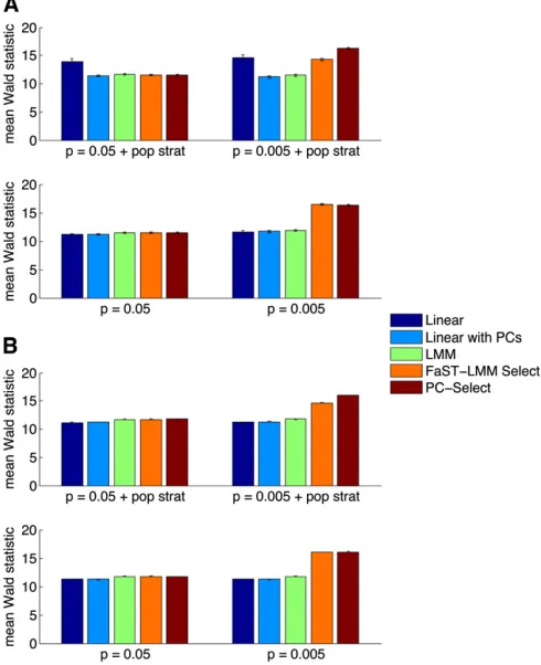
We found that when few SNPs were causal (P= 0.005), FaST-LMM Select inflated null statistics in the presence of population stratification (lGC= 1.2660.03), whereas PC-Select was properly calibrated (lGC= 1.0160.01) (Table 1). Moreover, FaST-LMM Select lost power in the presence of population stratification (measured by the mean Wald statistic on causal SNPs: 14.3 6 0.2 with stratification vs.

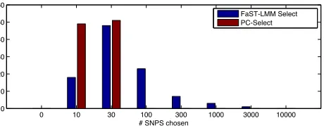
16.4 60.1 without), whereas PC-Select’s power in simula-tions with and without population stratification was not sig-nificantly different (16.360.1vs. 16.360.1) (Figure 1). Thus, even though PC-Select corrected for stratification, this advantage did not come at the expense of power. This gain is likely because the PCs reduce noise in selecting subsets of SNPs for the GRM in the presence of population stratifi ca-tion. In addition, PC-Select chose fewer SNPs than FaST-LMM Select to include in the GRM (over 100 simulations, mean SNPs chosen: 20 vs. 240, Figure S1), yielding potential computational savings. When many SNPs were

causal (P= 0.05), both methods used nearly all SNPs in the GRM (over 100 simulations, mean SNPs chosen:9400 and8800 of 10,000, respectively), achieving similar perfor-mance to standard LMM.

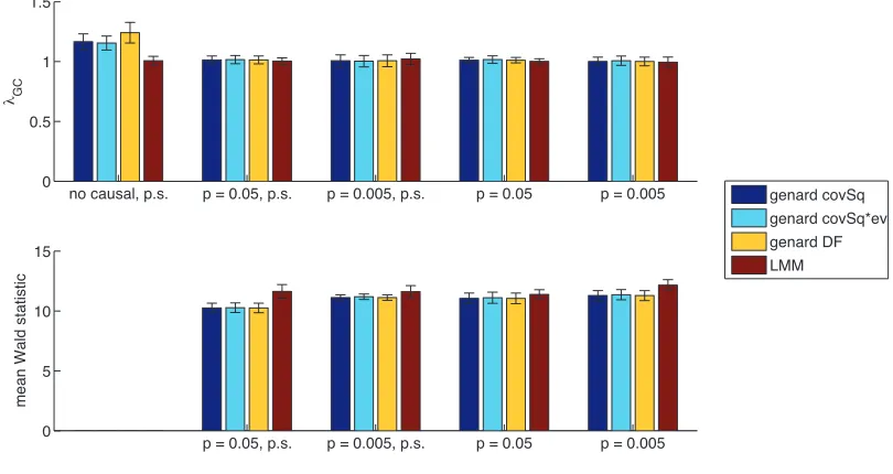
We also investigated a recent extension of FaST-LMM Select, thegenardmethod (Hoffman 2013) thatfits a data-adaptive low-rank GRM; however, we found that it did not have increased power over LMM in our simulations (Figure S5), which is consistent with previous simulations in a sim-ilar context (Hoffman 2013).

Next, we evaluated inflation and power on real genotypes with simulated phenotypes in a similar manner. We analy-zed 5000 individuals randomly subsampled from a multiple-sclerosis (MS) study genotyped on Illumina arrays (Sawcer

et al.2011) made available via Wellcome Trust Case Control Consortium 2 (WTCCC2) (see Materials and Methods). As before, we separated GRM SNPs and candidate SNPs to avoid proximal contamination and provide a fair comparison of methods. We randomly sampled 50,000 SNPs for the GRM from chromosomes 3 to 22, 250 causal SNPs from chromosome 1, and 500 null SNPs from chromosome 2. To simulate environmental variance aligned with population structure, we added 0.25 times the first PC (after the PC had been normalized to variance 1) to each individual’s phenotype. Otherwise, we generated phenotypes as be-fore and report simulations over 200 randomly generated phenotypes.

We again found that when few SNPs were causal (P= 0.005), FaST-LMM Select inflated null statistics in the pres-ence of population stratification (lGC = 1.06 6 0.01), whereas PC-Select was properly calibrated (lGC = 1.016 0.01) (Table 2). Moreover, FaST-LMM Select lost power in

Table 1 Extent of null statistic inflation as measured bylGC[median Wald statistic on test null SNPs divided by the theoretical median under the null distribution (Devlin and Roeder 1999)]

MeanlGC(SE) Pop. strat.,P= 0.05 Pop. strat.,P= 0.005 P= 0.05 P= 0.005

Linear regression 3.8 (0.4) 4.5 (0.5) 1.01 (0.01) 1.01 (0.01)

Linear regression with PCs 1.02 (0.01) 1.03 (0.01) 1.01 (0.01) 1.02 (0.01)

LMM 1.01 (0.01) 1.02 (0.01) 1.01 (0.01) 1.01 (0.01)

FaST-LMM Select 1.04 (0.01) 1.26 (0.03) 1.01 (0.01) 0.99 (0.01)

PC-Select 1.01 (0.01) 1.01 (0.01) 1.01 (0.01) 0.99 (0.01)

We tabulatelGCfor linear regression, linear regression with PCs, standard LMM, FaST-LMM Select, and PC-Select on simulated genotypes and phenotypes with and without

population stratification as the fraction of causal SNPs (P= 0.05, 0.005) varies. Values shown are meanlGCover 100 simulations with standard errors (SE) in parentheses.

FaST-LMM Select inflates statistics in the presence of population stratification when few SNPs are causal (P= 0.005), which may result in false positives. Pop. strat., population stratification.

Table 2 Extent of null statistic inflation measured bylGC

MeanlGC(SE) Pop. strat.,P= 0.05 Pop. strat.,P= 0.005 P= 0.05 P= 0.005

Linear regression 1.58 (0.02) 1.55 (0.02) 1.03 (0.01) 1.04 (0.01)

Linear regression with PCs 1.01 (0.01) 1.00 (0.01) 1.01 (0.01) 1.02 (0.01)

LMM 1.02 (0.01) 1.01 (0.01) 1.00 (0.01) 1.02 (0.01)

FaST-LMM Select 1.02 (0.01) 1.06 (0.01) 1.00 (0.01) 1.02 (0.01)

PC-Select 1.01 (0.01) 1.01 (0.01) 1.00 (0.01) 1.01 (0.01)

We tabulatelGCfor linear regression, linear regression with PCs, standard LMM, FaST-LMM Select, and PC-Select on real genotypes and simulated phenotypes with and

without population stratification as the fraction of causal SNPs (P= 0.05, 0.005) varies. Values shown are meanlGCover 200 simulations with standard errors (SE) in

parentheses. FaST-LMM Select inflates statistics in the presence of population stratification when few SNPs are causal (P= 0.005), which may result in false positives.

the presence of population stratification (measured by the mean Wald statistic on causal SNPs: 14.64 6 0.05 with stratification vs. 16.02 6 0.05 without); in contrast, PC-Select’s power in simulations with and without population stratification was not significantly different (16.02 6 0.05

vs. 16.0860.05) (Figure 1). In all of our simulations, PC-Select produced noninflated statistics and high power.

Finally, we analyzed data from 10,204 MS cases and 5429 controls genotyped on Illumina arrays (Sawcer et al.

2011) made available via WTCCC2 (seeMaterials and Meth-ods). The cases and controls were not matched for ancestry and thus exhibited substantial population stratification. Evaluated over all SNPs, PC-Select had lGC = 1.24 and FaST-LMM Select hadlGC = 1.20. Due to polygenicity, we expectlGCon all markers to be.1. On the same data, Yang

et al.(2014) reportlGC= 1.23 and 1.20 for linear regres-sion with PCs and LMM, respectively, which they show is consistent with polygenicity. To evaluate power, we consid-ered Wald statistics at 75 known associated SNPs (see Ma-terials and Methods and Table S1 for Wald statistics). PC-Select consistently gave larger Wald statistics than FaST-LMM Select (63 of 75 markers;P= 231029_{, mean}

Wald statistic 12.07 vs. 11.30). Based on cross-validation,

both PC-Select and FaST-LMM Select chose to use all markers. This may indicate that the disease is not caused by a small number of loci with large effects or that our sample size is too small to capture this effect. Although PC-Select and FaST-LMM Select chose to use all SNPs and thus neither method inflated statistics, we emphasize that withouta priori knowledge about the genetic architecture, PC-Select automatically tunes the number of SNPs to in-clude in the GRM to optimize power and simultaneously protects against population stratification at no cost to power. Janss et al. (2012) caution against using PCs as fixed effects in combination with a random effect derived from the GRM when estimating heritability. This may result in an ill-posed model because the PCs enter both as fixed effects and implicitly through the random effect. We avoid this issue when estimating variance components by using the PCs asfixed effects in a restricted maximum-likelihood (REML) approach, which projects the genotype matrix into a subspace orthogonal to the PCs, effectively removing them from the random effect. We also note that population struc-ture and PCs have previously been used successfully asfixed effects (or separate random effects) in mixed-model settings to address confounding from population structure and from unusually differentiated markers (Yuet al.2006; Zhaoet al.

2007; Priceet al.2010, 2013; Sul and Eskin 2013). Using PCs in a linear model does not correct for family relatedness and cryptic relatedness (Price et al. 2010). As suggested by Yang et al.(2014), due to the large length of segments shared identical-by-descent, using a subset of SNPs may correct for cryptic relatedness. Listgarten et al.

(2012) show that using a subset of SNPs in the GRM does not inflate statistics on the WTCCC data, where inflation is likely primarily due to cryptic relatedness. We expect that PC-Select will not be inflated by cryptic relatedness for the same reasons. In most human data sets with unrelated indi-viduals, family relatedness is not an issue; however, for data sets with strong family relatedness, we suspect there may be cases where both PC-Select and FaST-LMM Select inflate statistics.

PC-Select has the same asymptotic runtime as FaST-LMM Select, quadratic in the number of individuals and linear in the number of markers. In practice, the runtime for the additional step of computing the PCs for the genotype matrix is minimal because both methods require several spectral decompositions of matrices of nearly the same size for the cross-validation step. It should be noted that while the asymptotic runtime of PC-Select and FaST-LMM Select is the same as that of previously published exact LMM methods (Lippert et al. 2011; Zhou and Stephens 2012), the actual runtime of both methods is ostensibly longer by a factor of 10 due to the validation step. The cross-validation step is parallelizable, so in practice this is not a significant limitation.

Including PCs as fixed effects allows PC-Select to infer ancestry from all SNPs simultaneously, while at the same time maintaining the benefits of using a statistically chosen

Figure 1 (A and B) Comparison of power for linear regression, linear regression with PCs, standard LMM, FaST-LMM Select, and PC-Select on simulated genotypes and phenotypes (A) and real genotypes and simulated phenotypes (B) with and without population stratification as the fraction of casual SNPs (P= 0.05, 0.005) varies. To measure power, we plot the mean Wald statistic on test causal SNPs. In all cases, PC-Select has the highest power of the methods that do not inflate statistics.

subset of the SNPs to estimate the GRM (Listgarten et al.

2012; Lippertet al.2013). As we have shown, using a com-bination of PCs and a subset of SNPs in the GRM gives the best of both worlds.

Materials and Methods

MS data set

We analyzed data from 10,204 MS cases and 5429 controls [the National Blood Service (NBS) and the 1958 Birth Cohort (1958BC)] genotyped on Illumina arrays made available to researchers via WTCCC2 (http://wtccc.org.uk/

ccc2/). We follow the quality-control standards in Yang

et al.(2014). Although Sawceret al.(2011) analyzed United Kingdom (UK) and non-UK samples separately followed by meta-analysis in most of their analyses, the data made avail-able to researchers include both UK and non-UK cases but only UK controls. We retained all samples to maximize sam-ple size. We considered markers that were present in each of MS, NBS, and 1958BC data sets and removed markers with

.0.5% missing data, P, 0.01 for allele-frequency differ-ence between NBS and 1958BC,P,0.05 for deviation from Hardy–Weinberg equilibrium,P,0.05 for differential miss-ingness between cases and controls, or minor allele fre-quency ,0.1% in any data set, leaving 360,557 markers. The 75 known associated markers were defined by includ-ing, for each MS-associated marker listed in the National Human Genome Research Institute (NHGRI) GWAS catalog

(http://genome.gov/gwastudies/), a single best tag atr2_.

0.4 from the set of 360,557 markers if available.

Statistical methods

PC-Select follows a similar framework to that of FaST-LMM Select (Lippertet al.2011, 2013; Listgartenet al.2012). For completeness, we list the steps and equations we used.

First, we describe a method for computing association statistics, and then in subsequent sections we describe the steps of PC-Select.

Association statistics:The phenotypey, covariatesX, and genotypes W are mean centered. Additionally, each ge-notype is divided by p2ffiffiffiffiffiffiffiffiffiffiffiffiffiffiffiffiffiffiffiffi^pð12^pÞ; where ^p is the esti-mated minor allele frequency. Then the phenotype is modeled as

y¼Xaþuþe;

whereuNð0;s2

gKÞ; eNð0;s2eIÞ;ais a vector of weights for the covariates, and Kis the GRM. This model naturally leads to an association statistic based on the Wald statistic. To calculate the association statistic for SNPw, we addw

as a fixed-effect covariate to the previous model and test whether its coefficient is significantly different from 0. Spe-cifically, consider the model

y¼wbþXaþuþe;

wherebis the coefficient for the test SNP. We estimates2

g and s2

e by REML. The fixed-effect coefficients (b, a) are estimated by maximum likelihood.

It is straightforward to construct the Wald statistic to test whetherb6¼0. LetV¼s2

gKþs2eIandQ= [w;X]. Thenb^is equal to the first entry of (QT_V21_Q)21_QT_V21_{yand varðb}^_Þ

is equal to thefirst entry of (QT_V21_Q)21_{. The test statistic is}

^

b2

var

^

b;

which is asymptoticallyx2_{distributed with 1 d.f.}

PC-Select:

Now we describe the PC-Select method:

Step 1: Extracting PCs: We extract the top five PCs from a GRM formed using all of the genotype data,

WWT_{, to use as fixed-effect covariates. We use X} to denote the matrix of user-specified covariates and the topfive PCs.

Step 2: Ranking SNPs by linear regression: Second, we rank the SNPs by a linear regression test statistic. Linear regression test statistics are calculated byfixing s2

g to 0 and using the procedure described above to calculate Wald statistics.

Step 3: Determining the GRM: As in FaST-LMM Select, PC-Select uses a subset of the SNPs that are likely to be causal. In this step, we determinek, the number of top SNPs (as ranked in Step 2) to include in the GRM. We use 10-fold cross-validation on predictive log-likelihood to choose the number of top SNPs. We choosekfrom a list of user-defined possibilities (e.g.,k2 {100, 1000, 3000, 10,000, 30,000,. . .}). First, we randomly divide individuals into 10 equal groups or folds. For each foldi, we form a test set from the individuals in foldiand use the rest of the individuals as a training set. For each choice ofk, we consider a subset of the genotype matrix consisting only of the top kSNPs (the ranking of the SNPs is recomputed per fold, using the training data). For notational simplicity, we also refer to the reduced genotype matrix by W, and it will be clear from context if this refers to the full genotype matrix or a subset. Let Wi denote the genotypes from fold i and W2i represent the genotypes from the rest of the folds (similarly foryandX). We wish to evaluate the predictive log-likelihood ofyigiven the training information (y2i, X2i, Xi) to assess the predictive

power of using only the top k SNPs in the GRM. Specifically, to evaluate the predictive log-likelihood, we start by forming a GRM from the training set

W2iW₂Ti: Then we estimate s2g and s2e from the training set by REML. We estimate a by ML with these variance parameters fixed. Then under the model

y¼Xaþuþe;

whereuNð0;s2

gWWTÞandeNð0;s2eIÞ;the pre-dictive distribution of the phenotypes given the training parameters,yijy2i;W;a;s2g;s2e;is normally distributed with mean

s2

gWiW₂Ti

W₂iW₂Tis2gþs2eI ₂1

ðy₂i2X2iaÞ þXia

and covariance

WiWiTs2gþse2I2s2gWiW₂Ti 3W₂iWT₂is2gþs2eI

21 _W

2iWiTs2g:

This can be evaluated efficiently, using the spectral decompositions computed in the REML step (Lippert

et al.2011; Listgartenet al.2012). We average the predictive log-likelihood over each of the 10 folds and choose the k that gives the highest average log-likelihood.

Step 4: Calculating association statistics:Finally, with the num-ber of top SNPs to use in the GRMfixed, we calculate association statistics for each SNP. LetWbe the geno-type matrix using the topkSNPs chosen in the previous step. To avoid proximal contamination (Listgartenet al.

2012), we use a leave-one-chromosome-out procedure (Yanget al.2014). For each test SNPw(which is not necessarily inW), we exclude the chromosome includ-ing that SNP from the GRM and calculate the Wald statistic for w with this GRM. We do this efficiently by precomputing and storing the GRM, excluding each chromosome in turn.

Acknowledgments

We thank Po-Ru Loh, Sean Simmons, and Jian Peng for helpful discussions. This study makes use of data generated by the Wellcome Trust Case Control Consortium. This research was funded by National Institutes of Health grants R01 GM108348 and R01 HG006399.

Literature Cited

Devlin, B., and K. Roeder, 1999 Genomic control for association studies. Biometrics 55(4): 997_–1004.

Hoffman, G. E., 2013 Correcting for population structure and kin-ship using the linear mixed model: theory and extensions. PLoS ONE 8(10): e75707.

Janss, L., G. de los Campos, N. Sheehan, and D. Sorensen, 2012 Inferences from genomic models in stratified popula-tions. Genetics 192: 693–704.

Kang, H. M., N. A. Zaitlen, C. M. Wade, A. Kirby, D. Heckerman et al., 2008 Efficient control of population structure in model organism association mapping. Genetics 178: 1709–1723. Kang, H. M., J. H. Sul, N. A. Zaitlen, S.-y. Kong, N. B. Freimeret al.,

2010 Variance component model to account for sample struc-ture in genome-wide association studies. Nat. Genet. 42(4): 348–354.

Lippert, C., J. Listgarten, Y. Liu, C. M. Kadie, R. I. Davidsonet al., 2011 FaST linear mixed models for genome-wide association studies. Nat. Methods 8(10): 833_–835.

Lippert, C., G. Quon, E. Y. Kang, C. M. Kadie, J. Listgarteet al., 2013 The benefits of selecting phenotype-specific variants for applications of mixed models in genomics. Sci. Rep. 3: 1815. Listgarten, J., C. Lippert, C. M. Kadie, R. I. Davidson, E. Eskinet al.,

2012 Improved linear mixed models for genome-wide associ-ation studies. Nat. Methods 9(6): 525–526.

Patterson, N., A. L. Price, and D. Reich, 2006 Population structure and eigenanalysis. PLoS Genet. 2(12): e190.

Price, A. L., N. J. Patterson, R. M. Plenge, M. E. Weinblatt, N. A. Shadicket al., 2006 Principal components analysis corrects for stratification in genome-wide association studies. Nat. Genet. 38(8): 904–909.

Price, A. L., N. A. Zaitlen, D. Reich, and N. Patterson, 2010 New approaches to population stratification in genome-wide associ-ation studies. Nat. Rev. Genet. 11(7): 459–463.

Price, A. L., N. A. Zaitlen, D. Reich, and N. Patterson, 2013 Response to Sul and Eskin. Nat. Rev. Genet. 14(4): 300. Sawcer, S., G. Hellenthal, M. Pirinen, C. Spencer, N. Patsopoulos et al., 2011 Genetic risk and a primary role for cell-mediated immune mechanisms in multiple sclerosis. Nature 476(7359): 214–219.

Segura, V., B. J. Vilhjálmsson, A. Platt, A. Korte, . Seren et al., 2012 An efficient multi-locus mixed-model approach for ge-nome-wide association studies in structured populations. Nat. Genet. 44(7): 825–830.

Sul, J. H., and E. Eskin, 2013 Mixed models can correct for pop-ulation structure for genomic regions under selection. Nat. Rev. Genet. 14(4): 300.

Svishcheva, G. R., T. I. Axenovich, N. M. Belonogova, C. M. van Duijn, and Y. S. Aulchenko, 2012 Rapid variance components-based method for whole-genome association analysis. Nat. Genet. 44: 1166–1170.

Yang, J., N. A. Zaitlen, M. E. Goddard, P. M. Visscher, and A. L. Price, 2014 Advantages and pitfalls in the application of mixed-model association methods. Nat. Genet. 46(2): 100_–106. Yu, J., G. Pressoir, W. H. Briggs, I. V. Bi, M. Yamasaki et al., 2006 A uni_fied mixed-model method for association mapping that accounts for multiple levels of relatedness. Nat. Genet. 38(2): 203–208.

Zhao, K., M. J. Aranzana, S. Kim, C. Lister, C. Shindo et al., 2007 An Arabidopsis example of association mapping in struc-tured samples. PLoS Genet. 3(1): e4.

Zhou, X., and M. Stephens, 2012 Genome-wide efficient mixed-model analysis for association studies. Nat. Genet. 44(7): 821– 824.

Communicating editor: I. Hoeschele

GENETICS

Supporting Information http://www.genetics.org/lookup/suppl/doi:10.1534/genetics.114.164285/-/DC1

Improving the Power of GWAS and Avoiding

Confounding from Population Strati

fi

cation

with PC-Select

George Tucker, Alkes L. Price, and Bonnie Berger

FILE S1

SUPPORTING TEXT

Model performance as the number of top SNPs to include in the GRM is varied

We

investi-gated model performance as the number of top SNPs,

k

, to include in the GRM is varied. In the

following simulations, we compared using the top

k

SNPs in the GRM to a model using PCs with

the top

k

SNPs. The following analysis explores the intermediate choice that the FaST-LMM Select

and PC-Select methods have to make. Both methods use cross-validation predictive log-likelihood

to choose

k

.

In the presence of population stratification and without causal SNPs, we found that no choice

of top

k

SNPs is sufficient to correct for population stratification, except when all SNPs are used

in the GRM (Figure S2). This illustrates the tension between using a subset of SNPs in the GRM

to increase power and the need to use all SNPs to correct for population stratification. On the other

hand, when using PCs, statistics were not inflated for any choices of

k

.

In the absence of population stratification, including PCs does not compromise power. The

power when using PCs with the top

k

SNPs is not significantly different than when using the top

k

SNPs (Figure S3).

In the presence of population stratification and casual SNPs, we find that when few SNPs

are causal (

p

= 0

.

005

), using a subset of SNPs increases power over standard LMM as previously

reported (L

et al.

2013). However, in this regime, using the top

k

SNPs inflates null statistics

(Figure S4). With PCs, there were choices of

k

that improved power over standard LMM, while at

the same time avoiding inflating null statistics.

Implementation

We suggest implementing PC-Select by extracting PCs from the genotype data

using EIGENSOFT (P

et al.

2006) and then running FaST-LMM Select (L

et al.

2011;

L

et al.

2012; L

et al.

2013) with REML using the PCs as fixed effects.

For large datasets, we found that FaST-LMM Select exhausted our 170-GB memory limit, so

we provide a memory efficient MATLAB implementation of the cross-validation step to select

k

.

Then using GCTA (Y

et al.

2011), the SNPs can be sorted by linear regression p-value, a

truncated GRM using the top

k

SNPs can be formed, and association statistics can be computed

using GCTA mlma-loco with a GRM consisting only of the top

k

SNPs. In all steps, the PCs are

included as fixed effects as well as any additional covariates.

EIGENSOFT is available at:

http://www.hsph.harvard.edu/alkes-price/software/

FaST-LMM Select is available at:

http://research.microsoft.com/en-us/um/redmond/

projects/mscompbio/fastlmm/

MATLAB data simulators, analysis pipeline, and cross-validation implementation are available at:

http://groups.csail.mit.edu/cb/pc-select/

GCTA is available at:

http://www.complextraitgenomics.com/software/gcta/

download.html

LITERATURE CITED

H

, G. E., 2013 Correcting for Population Structure and Kinship Using the Linear Mixed

Model: Theory and Extensions. PloS ONE

8

(10)

:

e75707.

L

, C., J. L

, Y. L

, C. M. K

, R. I. D

, and D. H

,

2011 FaST linear mixed models for genome-wide association studies. Nature Methods

8

(10)

:

833–835.

L

, C., G. Q

, E. Y. K

, C. M. K

, J. L

, and D. H

,

2013 The benefits of selecting phenotype-specific variants for applications of mixed models in

genomics. Scientific Reports

3

.

L

, J., C. L

, C. M. K

, R. I. D

, E. E

, and D. H

-MAN

, 2012 Improved linear mixed models for genome-wide association studies. Nature

Meth-ods

9

(6)

:

525–526.

P

, A. L., N. J. P

, R. M. P

, M. E. W

, N. A. S

, and

D. R

, 2006 Principal components analysis corrects for stratification in genome-wide

association studies. Nature Genetics

38

(8)

:

904–909.

Y

, J., S. H. L

, M. E. G

, and P. M. V

, 2011 GCTA: a tool for

genome-wide complex trait analysis. The American Journal of Human Genetics

88

(1)

:

76–82.

10 12 14 16 18 20

Top Top w/ PCs

mean Wald

1 1.5 2

Top Top w/ PCs hGC

0 10 30 100 300 1000 3000 10000 0

10 20 30 40 50 60

# SNPS chosen

n_samples = 100, n = 1000, m = 10000, m_test = 50, m_null = 500 F_st = 0.05, trait diff = 0.25, sigma_e = 0, p = 0.005

FaST-LMM Select PC-Select

Figure S1.

Comparison of number of SNPs chosen by Fast-LMM Select and PC-Select. The histogram

shows the choices made by each method over

100

simulations with population stratification and

p

= 0

.

005

.

On average PC-Select chooses fewer SNPs to include in the GRM.

0 10 30 100 300 1000 3000 10000 0.8

1 1.2 1.4 1.6 1.8 2

# SNPs

GC

Stratification test with F_st = 0.05 n_samples = 100

n = 1000 m = 10000

Top SNPs Top SNPs with PCs

Figure S2.

Comparison of inflation when using the top

k

SNPs in the GRM and when using PCs with the

top

k

SNPs in the GRM. Two populations are simulated with

F

= 0

.

05

and no SNPs are causal. Without

PCs, the only choice of

k

that is not significantly inflated is using all SNPs. With PCs, no choice of

k

is

inflated.

0 10 30 100 300 1000 3000 10000 5

10 15 20

# SNPs

mean Wald statistic

p = 0.05

Top SNPs Top SNPs with PCs

0 10 30 100 300 1000 3000 10000

5 10 15 20 25

# SNPs

mean Wald statistic

p = 0.005 Top SNPs

Top SNPs with PCs

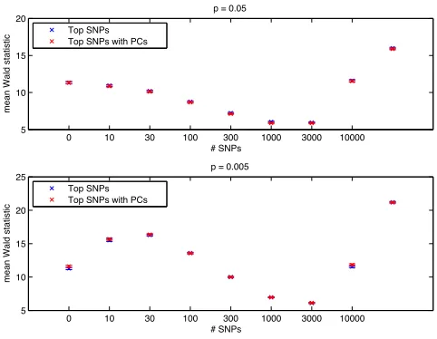
Figure S3.

Comparison of power when using the top

k

SNPs in the GRM and when using PCs with the

top

k

SNPs in the GRM. A fraction

p

= 0

.

05

,

0

.

005

of the SNPs were randomly chosen as causal and

population stratification was not present. The last unlabeled points result from using only truly causal SNPs

to construct the GRM. It represents the highest achievable score. In all cases, the power is not significantly

different between the two methods.

0 10 30 100 300 1000 3000 10000 5

10 15 20 25

# SNPs

mean Wald statistic

0 10 30 100 300 1000 3000 10000

0 1 2 3 4 5

# SNPs

λGC

Top SNPs Top SNPs with PCs

Top SNPs Top SNPs with PCs

Figure S4.

Comparison of power and

λ

when using the top

k

SNPs in the GRM and when using PCs

with the top

k

SNPs in the GRM. Two populations were simulated with

F

= 0

.

05

and a randomly chosen

fraction

p

= 0

.

005

of SNPs were chosen as causal. The top subplot measures power by mean Wald statistic

on test causal SNPs and the bottom subplot measures inflation by

λ

on an independent set of null test

SNPs. Whenever using the top

k

SNPs without PCs has higher power than using PCs, it also exhibits

significant inflation of

λ

.

no causal, p.s. p = 0.05, p.s. p = 0.005, p.s. p = 0.05 p = 0.005 0

0.5 1 1.5

λGC

p = 0.05, p.s. p = 0.005, p.s. p = 0.05 p = 0.005 0

5 10 15

mean Wald statistic

genard covSq genard covSq*ev genard DF LMM

Figure S5.

Comparison of

λ

and power for the genard method (H

2013) and standard LMM

on simulations with and without population stratification (abbreviated p.s.) as the fraction of casual SNPs

(no causal,

p

= 0

.

05

,

0

.

005

) varies. As recommended by the author of the genard method, model

complexity is selected by BIC and PCs are ordered by squared correlation to the phenotype (covSq),

squared correlation to the phenotype multiplied by the eigenvalue (covSq*ev), and effective degrees of

freedom (DF). In these simulations, genard does not provide a benefit over standard LMM.

10

SI

G.

Tucker

et

al.

Table S1   Wald statistics for 75 published associated markers in the MS data set.