Accounting for Sampling Error in Genetic Eigenvalues Using Random Matrix Theory

(1)

| INVESTIGATION

Accounting for Sampling Error in Genetic Eigenvalues

Using Random Matrix Theory

Jacqueline L. Sztepanacz1_{and Mark W. Blows} School of Biological Sciences, University of Queensland, St. Lucia, Queensland, Australia 4072

ABSTRACTThe distribution of genetic variance in multivariate phenotypes is characterized by the empirical spectral distribution of the eigenvalues of the genetic covariance matrix. Empirical estimates of genetic eigenvalues from random effects linear models are known to be overdispersed by sampling error, where large eigenvalues are biased upward, and small eigenvalues are biased downward. The overdispersion of the leading eigenvalues of sample covariance matrices have been demonstrated to conform to the Tracy–Widom (TW) distribution. Here we show that genetic eigenvalues estimated using restricted maximum likelihood (REML) in a multivariate random effects model with an unconstrained genetic covariance structure will also conform to the TW distribution after empirical scaling and centering. However, where estimation procedures using either REML or MCMC impose boundary constraints, the resulting genetic eigenvalues tend not be TW distributed. We show how using conﬁdence intervals from sampling distributions of genetic eigenvalues without reference to the TW distribution is insufﬁcient protection against mistaking sampling error as genetic variance, particularly when eigenvalues are small. By scaling such sampling distributions to the appropriate TW distribution, the critical value of the TW statistic can be used to determine if the magnitude of a genetic eigenvalue exceeds the sampling error for each eigenvalue in the spectral distribution of a given genetic covariance matrix.

KEYWORDSgenetic variance; eigenvalues; random matrix theory; Tracy–Widom distribution; REML-MVN

A

S a consequence of pleiotropy, the biological conclusions drawn from the distribution of genetic variance across phenotypic space are often in sharp contrast to the magnitude of genetic variance typically observed for individual traits (Dickerson 1955; Blows and Hoffmann 2005). Most individual traits tend to display substantial levels of genetic variance; however, most of this genetic variance is often conﬁned to fewer multivariate trait combinations than the number of in-dividual traits that are measured (Hine and Blows 2006; Kirkpatrick 2009; Walsh and Blows 2009). As applications of quantitative genetics to human health, agriculture, and evolu-tionary biology move toward adopting multivariate analyses of genetic variance, it will therefore be important that analytical approaches to accommodate the complexity of higher dimen-sional genetic information are developed.

The fundamental tool for understanding how pleiotropic covariance restricts the genetic variance in individual traits to multivariate combinations of these traits is the genetic

covariance (G) matrix, a symmetrical variance-component ma-trix whose diagonal elements represent the genetic variance in individual traits and the off-diagonal elements the covariances between them. The multivariate distribution of genetic vari-ance is then determined by the empirical spectral distribution of the eigenvalues ofG, in which each eigenvalue explains a portion of the total genetic variance underlying the phenotypic space (Dickerson 1955; Hill and Thompson 1978; Lande 1979; Pease and Bull 1988; Blows 2007). Although analyses of the spectral distribution ofGare relatively uncommon, an expo-nential decline in eigenvalues is typically observed, with some eigenvalues approaching zero (Kirkpatrick 2009; Pitcherset al. 2014). In evolutionary genetics the relative sizes of the eigen-values ofGare of particular interest, as they may determine how populations respond to selection in directions of pheno-typic space. For example, trait combinations with small genetic eigenvalues that have low levels of genetic variance form a nearly null genetic subspace (Gomulkiewicz and Houle 2009; Houle and Fierst 2013; Hineet al.2014), which may or may not include a true null subspace where genetic variance is zero (Mezey and Houle 2005). The response to selection in these directions of phenotypic space may be severely slowed (Kirkpatricket al.1990) and biased toward trait combinations Copyright © 2017 by the Genetics Society of America

doi:https://doi.org/10.1534/genetics.116.198606

Manuscript received December 4, 2016; accepted for publication April 17, 2017; published Early Online May 5, 2017.

1_{Corresponding author: School of Biological Sciences, University of Queensland, St.}

(2)

with higher levels of genetic variance (Chenowethet al.2010). If population sizes are small, failure to respond to selection in these regions of phenotypic space is also a real possibility (Gomulkiewicz and Houle 2009; Hine et al. 2014). Conse-quently, determining whether the eigenvalues from variance-component matrices that represent levels of genetic variance are signiﬁcantly different from zero is important for under-standing the evolution of multivariate phenotypes.

Although the pattern of decay in genetic eigenvalues from multivariate genetic analyses may reﬂect the biological covari-ance among traits, it is known from random matrix theory (RMT) that a similar pattern is also the expected outcome from random sampling alone (Johnstone 2006). RMT provides a framework for understanding the behavior of eigenvalues of symmetrical matrices with elements drawn randomly from a wide array of statistical distributions. For sample covariance matrices in par-ticular, the behavior of such eigenvalues has been the subject of intense interest (Wigner 1955; Bai and Silverstein 2010). In a genetics context, sample covariance matrices describe among-individual covariance structure, for example SNPs that are rep-resented as genomic relatedness matrices (Patterson et al. 2006), and phenotypic covariance matrices.

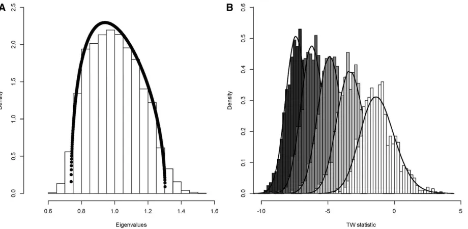
To illustrate two key results from RMT for sample covari-ance matrices, consider the phenotypic covaricovari-ance (P) matrix of a set ofp= 5 quantitative traits sampled from a multivar-iate normal distribution with a mean of 0 and covariance matrix equal to the identity matrix onn= 250 individuals. While the naive expectation would be that all eigenvalues of this matrix are equal to one, sampling error causes the eigen-values to be overdispersed, where some eigeneigen-values are

(3)

of RMT, and it has subsequently been conﬁrmed that the MP distribution can be generalized to describe the bulk distribu-tion of eigenvalues from variance component matrices (Fan and Johnstone 2016). In addition to the bulk distribution of eigenvalues, the leading eigenvalue ofGhas been shown to conform to the TW distribution using an empirical scaling approach (Saccentiet al.2011; Blows and McGuigan 2015), highlighting that hypothesis testing of genetic eigenvalues can take advantage of the TW distribution to form the appro-priate null distribution that observed genetic eigenvalues can be tested against.

Here, we show how RMT approaches can be applied in quan-titative genetic analyses to account for the sampling error that is concentrated in the leading eigenvalues ofGmatrices. We dem-onstrate how the use of conﬁdence intervals on the eigenvalues of G estimated from restricted maximum likelihood (REML) and Bayesian genetic analyses can result in erroneous conclusions con-cerning the presence of genetic variance when examined in the absence of the appropriate null distribution. We integrate the use of the TW distribution into the analyses of genetic eigenvalues from these approaches to enable a test of whether a genetic ei-genvalue signiﬁcantly differs from the null distribution.

Methods

Simulation of random data

To illustrate the behavior of the sampling variance in genetic eigenvalues, we generated 10,000 simulated data sets with a simple experimental design that represented 50 lines, with 5 individuals sampled from each line (representing, for exam-ple, 5 individuals sampled from each of 50 inbred lines). The identity matrix was used to sample theﬁve traits for each data set from a multivariate normal distribution with a mean of 0, giving no rise to within- or among-line covariance. Therefore, any covariance among theﬁve traits within each data set was solely a consequence of sampling. Estimation of (co)variance components at the among-line (genetic) level then represents the behavior of the sampling error in the genetic variance of individual traits and the multivariate genetic eigenvectors, in the absence of genetic information in the data.

This simulation closely matches that used in Blows and McGuigan (2015), where the relevance of the MP and TW distributions for genetic eigenvalues wasfirst explored using 10 simulated traits. In the current work we use onlyfive traits to reduce computational times. This also represents the modal number of traits that are currently used in empirical studies that have estimatedGmatrices (Pitcherset al.2014). While RMT was developed for very high-dimensional problems, the TW distribution has been shown to empiricallyfit well with p = 5 traits in a number of contexts (Ma 2012), including variance component matrices (Blows and McGuigan 2015).

Statistical analysis

The statistical analysis of multivariate genetic data typically employs either REML- or Bayesian-based approaches to esti-mate the genetic covariance matrix. In these analyses, an

important choice to be made in the multivariate modeling is the type of covariance structure to be imposed on the data at the genetic level (in this case the among-line level of our simulation). The simplest covariance structure is an uncon-strained covariance matrix that permits genetic correlations to exceed the theoretical boundary (21 and 1), often resulting in negative eigenvalues of G. The probability that an esti-matedGmatrix will be nonpositive deﬁnite is very high with the commonly employed sample sizes in evolutionary studies (Hill and Thompson 1978). While negative eigenvalues seem counterintuitive, they are an important component of the behavior of the sampling error in variance component matri-ces and the unconstrained covariance structure is therefore most compatible with RMT (Blows and McGuigan 2015).

An alternative choice that is used extensively in quantita-tive genetics is a constrained covariance structure that re-quires the estimate ofGto stay within the parameter space. Within REML-based analyses, this can be achieved by speci-fying a factor-analytic covariance structure thatfits a number of orthogonal trait combinations, up to the number of traits. In this case,Gis constrained to be positive semidefinite, so that all eigenvalues are greater than zero. Similarly, Bayesian analyses that use Markov chain Monte Carlo (MCMC) typi-cally sample from a sums-of-squares-and-cross-product ma-trix, and consequently estimates ofGfrom these analyses are also constrained to be positive semidefinite (Hazelton and Gurrin 2003; Sorensen and Gianola 2010). Although a con-strained covariance structure results in biologically sensible estimates ofG, the leading genetic eigenvalues remain sub-ject to the sampling error predicted from RMT as we show below.

(4)

experimental designs that represent different levels of power, and we demonstrate how REML-MVN sampling can be used to test whether a genetic eigenvalue represents a signiﬁcant level of genetic variance using the TW distribution.

REML estimation of G using unstructured and factor-analytic models and the TW distribution

We performed two separate analyses of the 10,000 simulated data sets,ﬁrst employing an unconstrained covariance struc-ture and second using a factor-analytic covariance strucstruc-ture. For both analyses,Gwas estimated using the following mul-tivariate linear model:

Y¼mþZluGþIe; (1)

where Ydenotes a stacked vector of multivariate observa-tions,Zlwas the among-line design matrix relating observa-tions to the vector of unknown random effects,uG was the vector of unknown random genetic effects, andewas a vector of residual errors. The random effect (and residuals) were assumed to be normally distributed and elements ofuGwere further assumed to be drawn fromu_GNð0;G5ZlÞ;where Gwas the genetic covariance matrix andZlwas the genetic relationship matrix. In the case of the unconstrained analysis, Gwas modeled as an unstructured covariance matrix; and in the case of the factor-analytic analysis,Gwas modeled using a full-rank, factor-analytic structure:

G¼LLT_;

(2)

where L was a lower triangular matrix of factor loadings. Models were run using REML implemented in the MIXED procedure in SAS (version 9.4; SAS Institute). Both analyses returned 10,000Gmatrices, from which the spectral decom-position provided 10,000 samples for each of theﬁve eigen-values of G. As any covariance inG estimated from these models is simply a consequence of sampling, these eigen-values form the null distribution of sampling variance that can be compared against the theoretical TW distribution.

To determine whether the eigenvalues ofGobtained from (1) conform to the TW distribution speciﬁc to each eigen-value, theyﬁrst needed to be scaled and centered. The scaling and centering parameters for the theoretical limiting dis-tributions of variance component matrices such as G are currently unknown (I. Johnstone, personal communication), however an empirical scaling approach can be used (Saccenti et al.2011).

Rescaling of each observed genetic eigenvaluelowas ac-complished using the approach of Saccentiet al.(2011):

TWG¼miþ si

soðlo2moÞ;

(3)

wheremiandsiare the mean and SD of the theoretical TW distribution for the ith eigenvalue, and mo and so are the mean and SD of the corresponding observed genetic eigen-values of random datalo;respectively. The rescaling proce-dure followed here differs from that given in Box 2 of Blows

and McGuigan (2015), with the removal of a redundant step represented by an initial rescaling using the equation TWw¼pð2=3Þ_ð_l_i₂₂_Þ_{before applying (3).}

To obtain the theoretical distributions of each eigenvalue to compare theTWGstatistic to, we generated 10,000 obser-vations from each theoretical TW distribution using its gamma approximation. For each theoretical TW distribution with meanðmiÞ;varianceðsiÞ;and skewnessðriÞ;the shape ðkiÞ; scale ðuiÞ; and constant ðaiÞ of the matching gamma distributionðG½ki;ui2aiÞis given by (Chiani 2014):

ki¼

4

r2

i

; ui¼siri

2 ; ai¼kiui2mi: (4)

The distributions of theTWGstatistics for the observed ge-netic eigenvalues were then compared to the appropriate theoretical TW distribution for that particular eigenvalue us-ing quantile–quantile (QQ) plots.

MCMC estimation of G and the TW distribution

MCMC is an analytical approach that is often used to place confidence on genetic parameters by sampling from the MCMC chain and using this posterior distribution of the (co)variance components to generate confidence intervals (O’Haraet al.2008; Sorensen 2008; Hadfieldet al.2010). The covariance components in such models are constrained to fall within the parameter space and hence the estimatedG matrices will be positive-definite (Hazelton and Gurrin 2003; O’Haraet al.2008; Hadfield 2010). Therefore, the posterior distribution cannot be used to test whether genetic variances themselves differ from zero. Consequently, a randomization of the data across the pedigree or with respect to the genetic groups, such that any estimated covariance is a consequence of sampling and not genetic variance, has been used to pro-vide a posterior null distribution that the observed distribu-tion is then compared to (e.g., Hadfield 2010; Aguirreet al. 2014; McGuiganet al.2015). To determine whether the ei-genvalues from the posterior null distribution generated by MCMC analyses conformed to the TW distribution, we ana-lyzed a single random data set (thefirst of our 10,000 simu-lated data sets from above) using the MCMCglmm package (Hadfield 2010) in R. We sampled from the posterior distri-bution of the MCMC chain 10,000 times, to obtain 10,000G matrices (and consequently 10,000 samples of each eigen-value). The analysis was repeated 10 times (for 10 different random data sets) to determine the consistency of results across the 10 data sets.

(5)

uninformative flat prior distributions have been shown to strongly influence (some) model parameters, and specifying uninformative priors at all scales of the analysis may be difficult (Van Dongen 2006; O’Hara et al.2008). Here we used two priors that are often employed in quantitative ge-netic studies: an inverse-Wishart distribution where the phe-notypic variance is partitioned equally among random effects and the degree of belief is weak (e.g., Wilsonet al.2010), and a half-Cauchy parameter-expanded prior that may perform better when variances are close to zero (e.g., Hadfield 2016). Preliminary analyses in which we used an improper prior deviated substantially from the TW distribution and often suffered from numerical issues, and therefore we do not con-sider this option any further.

In both cases, the priors for the location parameters were normally distributed and diffuse about a mean of 0 and a variance of 108_:_{For the variance components we} _fi_rst ana-lyzed the data using an inverse-Wishart prior where the scale parameter was defined by a diagonal matrix containing val-ues of one-half of the phenotypic variance, and the degree of belief was set at 5.002, slightly more than the dimensions of the matrix. Next, we used a half-Cauchy parameter-expanded prior with a scale parameter equal topffiffiffiffiffiffiffiffiffiffiffi5000:For both priors the joint posterior distribution was estimated from 3,000,000 MCMC iterations sampled at 300 iteration intervals after an initial burn-in period of 300,000 iterations. Overall, model convergence diagnostics indicated that the MCMC chain sam-pled the parameter space adequately, and the autocorrelation between successive samples was typically much below 0.1 for analyses using both priors.

For each of 10,000 samples of the posterior distribution, we performed an eigenanalysis ofG, obtaining 10,000 samples for each eigenvalue. We subsequently scaled the eigenvalues as above, according to Equation 3, and theTWGstatistics for the genetic eigenvalues were then compared to the appropri-ate gamma approximation of the theoretical TW distribution for that particular eigenvalue.

REML estimation of G with MVN sampling and the TW distribution

Conceptually similar to the confidence intervals placed on variance component estimates from MCMC using the poste-rior distribution, Houle and Meyer (Meyer and Houle 2013; Houle and Meyer 2015) have recently shown how the inverse of the Fisher information matrix of covariance parameters ½HðuGÞ21 from multivariate REML models can be used to generate confidence intervals on REML estimates of variance components. This approach is appealing compared to MCMC methods from both a computational perspective and because no prior specification is required. To determine whether the sampling distribution of the eigenvalues generated by REML-MVN sampling conformed to the TW distribution, we analyzed a single random data set (thefirst of the 10,000 simulated data sets from above), fitting an unconstrained REML analysis in accordance with (1), and then obtained 10,000 REML-MVN samples from the inverse of the Fisher

information matrix½HðuGÞ21of this analysis. Again, we re-peated the analysis 10 times (for 10 different random data sets), to determine the consistency of results across data sets. REML estimates of the p(p+ 1)/2 (co)variance compo-nents were obtained by fitting (1) with an unconstrained covariance structure that allowed negative eigenvalues. Fol-lowing estimation of the (co)variance components, we di-rectly sampled the elements of G 10,000 times, from the distributionN½u^_G; Hðû_GÞ21;whereû_Gwas the vector of pa-rameter estimates of G and HðûGÞ was the inverse of the Fisher information matrix from the unconstrained analysis (Meyer and Houle 2013; Houle and Meyer 2015). This is considered sampling on theG-scale of an unconstrained anal-ysis. Alternatively, one can sample on theL-scale, where the elements ofL(with vector of estimatesuLÞare the Cholesky factors from a factor-analytic model. However, REML-MVN sampling requires that the Fisher information matrix be safely positive-definite. The Fisher information matrix from the analysis of these data that employed a factor-analytic covariance structure was highly ill-conditioned, and conse-quently did not meet this requirement. Therefore, we only sample on theG-scale of unconstrained analyses here.

For each of the 10,000 samples from the distribution N½^uG; Hð^uGÞ21;we performed an eigenanalysis ofG, obtain-ing 10,000 estimates of each eigenvalue. We subsequently scaled the eigenvalues as above, according to Equation 3, and theTWGstatistics for the genetic eigenvalues were then compared to the appropriate gamma approximation of the theoretical TW distribution for that particular eigenvalue.

Using REML-MVN to test observed genetic eigenvalues against the appropriate null

To illustrate how the REML-MVN approach can be used to test whether genetic eigenvalues signiﬁcantly differ from the null distribution, we simulated two data structures that incorpo-rated known genetic variance for each of three experimental designs that represented different levels of power. Incorpo-rating known genetic variance into the simulation also allowed us to highlight the potential problems that arise when REML-MVN sampling is used to generate conﬁdence intervals on eigenvalues without reference to the TW distribution.

The three experimental designs were: 50 lines with 5 indi-viduals sampled per line (the same design presented above for random data); 500 lines with 10 individuals sampled per line; and a half-sibling design with 200 sires, 5 dams per sire, and 5 individuals per full-sibling family. These experimental designs represent, for example, 50 (500) inbred lines with 5 (10) individuals sampled per line, and a standard half-sibling breed-ing design used in many quantitative genetic studies.

(6)

L1¼ 0 B B B B @

0:8 0 0 0 0 0:7 0 0 0 0 0:6 0 0 0 0 0:5 0 0 0 0 0:4 0 0 0 0

1 C C C C A;

together with an unstructured dam (in the case of the half-sib design) and residual (for all cases) covariance matrix that resulted in an expected eigenvalue ofl1of 0.56. The among-line covari-ance matrixG5 for the data simulated to haveﬁve genetic di-mensions was modeled using the factor-analytic structure:

L5¼ 0 B B B B @

0:8 0 0 0 0

0:7 20:9 0 0 0

0:6 0:3 20:4 0 0 0:5 20:6 20:7 0:3 0 0:4 0:5 0:8 20:1 0:4

1 C C C C A;

together with an unstructured dam (in the case of the half-sib design) and residual (for all cases) covariance matrix. The expected eigenvalues of the ﬁve genetic factors were 0.69, 0.57, 0.32, 0.08, and 0.01, respectively.

For each of the three experimental designs, we also sim-ulated random data using the identity matrix to sample from a multivariate normal distribution with a mean of 0, giving rise to no within- or among-line covariance. This provided a baseline with which the performance of REML-MVN in con-junction with the TW could be compared for experimental designs with varying levels of power. In total there were three experimental designs, two simulated data sets with genetic variance, and one simulated random data set (six data sets with genetic variance plus three data sets without genetic variance).

To obtain the parameter estimates of the“observed”Gfor each experimental design/data set combination that had ge-netic variance, each of the six data sets were analyzed using model (1) with an unconstrained covariance structure. To generate their respective null distributions, the data were randomized across the lines (or sires in the case of the half-sib design), and again were analyzed using model (1) with an unconstrained covariance structure. We then sampled the (co)variance elements of the randomized G 10,000 times, from the distribution N½u^G; Hð^uGÞ21 (Meyer and Houle 2013; Houle and Meyer 2015).

The genetic eigenvalues that formed the null distributions were scaled using (3). To compare the eigenvalues resulting from the observedGto the null distribution, they also needed to be placed on the appropriate scale. For each observed eigenvalue, the TWG statistic was calculated according to (3) where mo and so were the mean and SD of the eigen-values from the null distribution of randomized data, sub-stituting each of the ﬁve observed genetic eigenvalues li for the observed distribution with genetic variance. The sam-pling distributions of the simulated random data for each of the three experimental designs were generated as described above.

Data availability

The authors state that all data necessary for conﬁrming the conclusions presented in the article are represented fully within the article.

Results

REML estimation of G using unstructured and factor-analytic models and the TW distribution

For the 10,000 random data sets, the magnitudes of the leading eigenvalues ofGwere biased upward by the concen-tration of sampling error under both the unconstrained and constrained models. Since these data were simulated ran-domly with respect to genetic line, the genetic variance in each trait and consequently in any eigenvector is expected to be zero. The average eigenvalues for l1 of 0.13 and 0.11, respectively, therefore represented spurious genetic variance that was purely a consequence of sampling error. With sam-ple covariance matrices, it is well known that as the ratio of the number of parameters to the number of observations ðp=nÞincreases, the inﬂation of the leading eigenvalues will also increase (Johnstone 2001). Therefore, we expect that the magnitude of the spurious eigenvalue will increase as the ratio of p to the genetic degrees of freedom increases, although this remains to be explored in detail for different experimental designs.

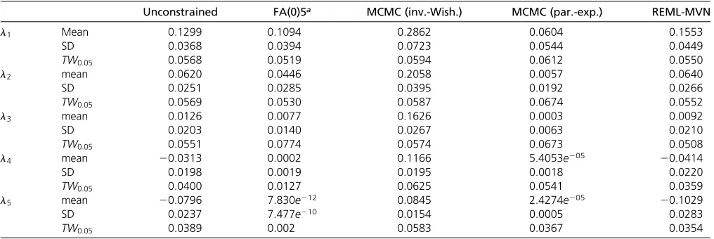
Each of theﬁrst four eigenvalues that were estimated from the 10,000 random data sets using an unconstrained covari-ance structure that permitted negative eigenvaluesﬁt the TW distribution well (Table 1). However, the last eigenvalue did show some deviation, falling below the 1:1 line on the QQ plot at the tails of the distribution (Figure 2 and Table 1). Consequently, the proportion of eigenvalues that exceeded the critical value of the theoretical distribution ata0:05was only 0.0389 (Table 1).

In contrast to the unstructured REML analyses, only the first two genetic eigenvalues from the modelfitting the factor-analytic structure appear to conform to the TW distribution (Figure 2 and Table 1). The factor-analytic covariance struc-ture constrains the genetic estimates to the parameter space, and therefore the lower bound on the eigenvalues from these models is zero. By the second eigenvalueðl2Þ;the effect of the boundary constraint was becoming evident by the devia-tion of the lower tail from the 1:1 line on the QQ plot (Figure 2B). As the boundary was approached, there was a significant deviation from the TW distribution for the last three eigen-values, evidenced by both the QQ plot (Figure 2, C–E) and the proportion of observations that exceeded the critical value (Table 1).

MCMC estimation of G and the TW distribution

(7)

along the x-axis is therefore determined by the individual data set that is used. For example, in theﬁrst of our simulated data sets, the observed lead eigenvalue estimated from an unconstrained REML analysis of that data set was 0.1084. Therefore it would be expected that the 10,000 samples of the posterior distribution from the MCMC analysis of this data set would center on 0.1084. However, the MCMC anal-yses returned posterior distributions of eigenvalues that sub-stantially differed in mode depending on the prior that was used. For the inverse-Wishart prior, the posterior distribution of the leading eigenvalueðl1Þwas centered on 0.2862, well above the parameter estimate from REML (Table 1). In con-trast, the parameter-expanded prior returned a posterior dis-tribution that was centered well below the REML parameter estimate at 0.0604 (Table 1).

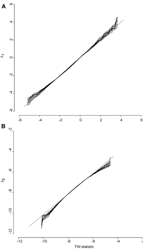
The posterior distributions of the eigenvalues from theﬁrst data set that was analyzed deviated substantially from the TW distribution for both priors that were used, with a larger pro-portion of eigenvalues exceeding the critical value than expected by chance in most cases (Table 1). This deviation from the theoretical distribution was consistent across all 10 of the ran-dom data sets that were analyzed (Figure 3, A and B).

The posterior distributions of variances from MCMC mod-els are constrained to fall within the parameter space, as they are for factor-analytic REML models, and therefore both the boundary constraint and the concentration of sampling var-iance in leading eigenvalues may result in their overestimation and consequent deviation from the theoretical distribution. However, considering that theﬁrst eigenvalue from MCMC models already failed to conform well to the TW distribution, despite being well away from the boundary withp= 5 traits, the boundary constraint may not be the only contributing factor to the deviation from the TW distribution in this case (Figure 3, A and B and Table 1).

REML estimation of G with MVN sampling and the TW distribution

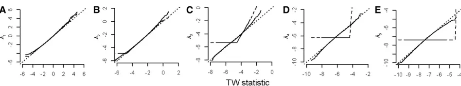
The REML-MVN sampling was carried out using the same 10 data sets analyzed in the MCMC models above. Again, for theﬁrst of the simulated data sets, the mean magnitude of the lead eigenvalue observed from the REML-MVN sam-pling approach was higher than the parameter estimate of 0.1084, with an average eigenvalue of 0.15 (Table 1). Despite the difference in mean for the lead eigenvaluel1;the sam-pling distribution generated by the REML-MVN approach conformed well to the TW distribution and in a consistent manner across the 10 data sets (Figure 4A), with the pro-portion of observations for theﬁrst data set that exceeded the critical value ða0:05Þ at 0.0469. Similarly, the following two eigenvaluesl2andl3 also conformed well to the theo-retical distribution (Table 1), at least as well as the eigen-values estimated from 10,000 random data sets using an unstructured covariance structure. However, the last eigen-valuel5deviated from the distribution, falling below the 1:1 line on the QQ plot at the tails of the distribution (Table 1) in a consistent manner across the 10 data sets (Figure 4B). This bias of the last eigenvalue was similar in magnitude to the bias observed from the analysis of 10,000 random data sets using an unstructured model (Table 1).

Using REML-MVN to test observed genetic eigenvalues against the appropriate null

It has recently been suggested that the conﬁdence intervals on genetic variances that are generated using REML-MVN can be used to determine whether eigenvalues contain nonzero levels of genetic variance by comparing the parameter esti-mate to the number of SDs above zero (Houle and Meyer 2015). For the REML-MVN analysis of the ﬁrst random data set, the observed mean of the leading eigenvalue was Table 1 The mean (posterior mode), SD, and proportion of samples exceeding the critical value for each eigenvalue

Unconstrained FA(0)5a MCMC (inv.-Wish.) MCMC (par.-exp.) REML-MVN

l1 Mean 0.1299 0.1094 0.2862 0.0604 0.1553

SD 0.0368 0.0394 0.0723 0.0544 0.0449

TW0:05 0.0568 0.0519 0.0594 0.0612 0.0550

l2 mean 0.0620 0.0446 0.2058 0.0057 0.0640

SD 0.0251 0.0285 0.0395 0.0192 0.0266

TW0:05 0.0569 0.0530 0.0587 0.0674 0.0552

l3 mean 0.0126 0.0077 0.1626 0.0003 0.0092

SD 0.0203 0.0140 0.0267 0.0063 0.0210

TW0:05 0.0551 0.0774 0.0574 0.0673 0.0508

l4 mean 20.0313 0.0002 0.1166 5.4053e205 20.0414

SD 0.0198 0.0019 0.0195 0.0018 0.0220

TW0:05 0.0400 0.0127 0.0625 0.0541 0.0359

l5 mean 20.0796 7.830e212 0.0845 2.4274e205 20.1029

SD 0.0237 7.477e210 _0.0154 _0.0005 _0.0283

TW0:05 0.0389 0.002 0.0583 0.0367 0.0354

The mean (or posterior mode in the case of MCMC samples), SD, and proportion of samples exceeding the critical value for each eigenvalue (li) of the analysis of either 10,000 data sets (unconstrained andﬁve-dimension factor-analytic modela_{) or 10,000 samples from a single data set (MCMC and REML-MVN). MCMC analyses were} conducted using either an inverse-Wishart prior (inv-Wish) or a parameter-expanded prior (par-exp). Approximate critical values for the TW statistic were determined by the 950,000th sample of the gamma approximation for each eigenvalueðl12l5Þ;and are 0.9748,21.5411,23.3005,24.7620, and26.0540, respectively. FA(0)5,ﬁ ve-dimension factor-analytic model; inv.-Wish., inverse-Wishart prior; par.-exp., parameter-expanded prior.

(8)

3.5-times larger than its SD and above zero (Table 1), rais-ing the possibility that samplrais-ing error could be misinter-preted as genetic variance in this dimension. Relying solely on the distribution of sampling error around an ei-genvalue generated by REML-MVN to infer genetic variance in real data will therefore likely be insufﬁcient to demon-strate the presence of genetic variance. However, the cen-tering and scaling parameters of the TW distributions speciﬁc to each eigenvalue can be used to form the appro-priate null distribution against which the observed genetic eigenvalues can be tested.

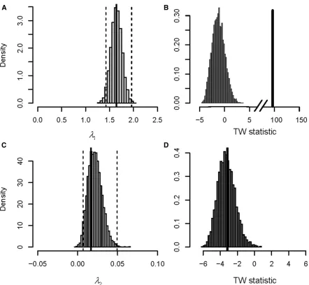
We simulated data to have either one genetic dimension or five genetic dimensions for each of three different experimen-tal designs (50 lines, 500 lines, 200 sires) representing dif-ferent levels of experimental power, to demonstrate how significance testing using REML-MVN sampling combined with the TW distribution performs in these situations. As expected, as the ratio ofpto the genetic degrees of freedom decreased, the inflation of the leading eigenvalues of random data simulated with no genetic variance decreased (Table 2). However, for all three experimental designs, the lower con-fidence interval for thefirst two eigenvalues of random data were above zero, despite the lack of simulated genetic vari-ance in these eigenvectors. This potentially indicates the presence of significant genetic variance when the confidence intervals are interpreted in isolation. When empirically rescaled to the TW distribution, however, none of the five eigenvalues were deemed significant by comparison of their TWGstatistics to the critical values of the TW distributions specific to each eigenvalue (Table 2), highlighting the value of the TW approach to test for the significance of observed genetic eigenvalues.

For the data simulated to have a single genetic eigenvalue, the lower confidence interval of the sampling distribution generated by REML-MVN forl1was far above zero at 1.2080, 1.6788, and 1.4224 for the 50 line, 200 sire, and 500 line cases, respectively (Table 2). Therefore, the presence of this genetic dimension was correctly identified by examining the confidence interval for all three experimental designs in this case. However, as observed for the random data, the lower confidence intervals ofl2 were also above zero, incorrectly identifying the presence of a second genetic dimension (Table 2). To illustrate this behavior, consider the example

of the 500 line experimental design. For bothl1andl2the mean unscaled eigenvalues were both above zero, and the 95% confidence intervals did not overlap zero (Figure 5, A and C), suggesting the presence of significant genetic var-iance. However, by empirically rescaling to the TW distri-bution, l1 was demonstrated to be the only significant genetic eigenvalue (Figure 5, B and D). Here the appropri-ate comparison was between the observed genetic eigen-value in real data and the null distribution generated by REML-MVN sampling of randomized data, after both the observed eigenvalue and null distribution were centered and scaled according to the theoretical TW distribution specific to that eigenvalue. The observed genetic eigen-value l1 fell well outside the null distribution (Figure 5B), and above the critical value of 0.987 (Table 1), indicating significant genetic variance in this genetic dimension. In con-trast, the observed eigenvaluel2fell well within the null dis-tribution (Figure 5D) and below the critical value of21.5411, indicating a lack of significant genetic variance in this dimension. Currently, the best method to test whether eigenvalues are significantly different from zero is by comparing the likeli-hoods of a series of nested reduced-rank, factor-analytic models. Here, if reducing the rank of the model from k to k21 dimensions significantly reduces the fit, then thekth eigenvalue is said to be significant (Hine and Blows 2006). For the 50 line, 200 sire, and 500 line simulated data sets with a single genetic eigenvalue, factor-analytic modeling identified a single genetic dimension in each (Table 2), con-sistent with the results of the TW approach presented above. Therefore, the TW approach performed as well as factor-analytic modeling in this case. For the data simulated to be full rank, factor-analytic modeling identified the presence of thefirst four genetic factors (Table 2). The lack of statistical support forl5was not surprising considering the low level of genetic variance accounted for by this factorðl5¼0:01Þ;and that factor-analytic models tend to be conservative. In con-trast, the TW testing approach correctly identified the pres-ence of allfive genetic eigenvalues (Table 2). However, the statistical significance ofl5should be interpreted with some caution. We previously demonstrated using REML-MVN sam-pling of random data (50 line experimental design) that the sampling distribution of the last eigenvalue did not conform well to the TW distribution (Figure 4B), with fewer samples Figure 2 (A–E) QQ plots of theTWGstatistics for thefive observed genetic eigenvaluesl12l5;respectively, from 10,000 simulated data sets, against

the approximations of their respective theoretical TW distributions. The solid lines depict theTWGstatistics from REML analyses that employed an

unconstrained covariance structure, whereas the dashed lines depict theTWGstatistics from factor-analytic models that constrain estimates ofGto the

(9)

exceeding the critical value than expected by chance (Table 1). This may result in anticonservative signiﬁcance tests for the last eigenvalue of variance component matrices.

Discussion

Sampling error generates patterns in the empirical spectral distribution of variance component matrices that can look strikingly like the biological patterns that are interpreted to represent genetic covariance, which concentrates genetic variance into fewer multivariate dimensions than the number of traits measured (Blows and McGuigan 2015). As a conse-quence of the magnitude of sampling error in the leading eigenvalues ofG, particular care needs to be taken to deter-mine if a genetic eigenvalue is greater in magnitude than

expected by sampling error alone. RMT provides a generally applicable framework for testing whether eigenvalues of sample covariance matrices represent signiﬁcant levels of variance (Tracy and Widom 1996, 2009; Johnstone 2001). Here we demonstrate that RMT can similarly be applied to the outcomes of multivariate genetic analyses that take the form of variance component matrices, to test whether leading genetic eigenvalues represent signiﬁcant levels of genetic variance.

Figure 4 (A) QQ plot of theTWGstatistic for theﬁrst genetic eigenvalue

vs. the theoretical TW distribution. The TWG statistic was calculated

according to (3), using the sampling estimates obtained from REML-MVN sampling of a model that employed an unconstrained covariance structure. The 10 lines represent the 10 data sets that were analyzed, and the dashed line indicates the 1:1 line. (B) QQ plot of theTWGstatistic for

theﬁfth genetic eigenvaluevs.the theoretical TW distribution. TheTWG

statistic was calculated according to (3), using the sampling estimates obtained from REML-MVN sampling of a model that employed an un-constrained covariance structure. The 10 lines represent the 10 data sets that were analyzed, and the dashed line indicates the 1:1 line. Figure 3 (A) QQ plot of theTWGstatistic for theﬁrst genetic eigenvalue

vs. the theoretical TW distribution. The TWG statistic was calculated

according to (3), using the posterior distribution of MCMC analyses that employed an inverse-Wishart prior. The 10 lines represent the 10 data sets that were analyzed, and the dashed line indicates the 1:1 line. (B) QQ plot of theTWGstatisticvs.the theoretical TW distribution as described

(10)

Sampling error in genetic eigenvalues of random data

In general, the genetic eigenvalues from unconstrained REML-based analyses of random data conformed well to the TW dis-tribution (Figure 2), with the small number of lines (n= 50) and traits (p= 5). While the proportion of leadingðl1Þ eigen-values that exceeded the critical value ata0:05 was.0.05 at 0.0568; as the number of genetic degrees of freedom andp increase, thefit to the theoretical distribution is predicted to further improve. This is illustrated, in part, by the betterfit of the sampling error ofl1to the theoretical distribution from the analysis of 200 random data sets ofp= 10 traits, where the proportion of eigenvalues exceeding the critical value was 0.05 (Blows and McGuigan 2015). While sampling error is known to concentrate genetic variance in the leading eigenvalues of G, particularly with the small sample sizes that are used here, the corollary is that the trailing eigenvalues must be under-estimated. In contrast to the leading eigenvalues, the last ei-genvaluel5did show some deviation from the theoretical TW distribution (Table 1), with a smaller proportion of eigen-values exceeding the critical value than expected by chance. The behavior of the last eigenvalue of sample covariance ma-trices may be better described by a reflected TW distribution (Ma 2012). Whether this may also be the case for variance component matrices such as G remains to be determined, and will be an important component of future studies.

In contrast to the goodfit to the TW distribution of the sampling error in eigenvalues from the unconstrained models, the sampling distribution of eigenvalues generated by factor-analytic models failed to conform to the TW distribution in general (Table 1). Currently, factor-analytic modeling is the best approach for testing whether eigenvalues significantly differ from zero, and is a useful tool in many cases that pro-vides biologically sensible estimates ofG. In this approach, a series of nested reduced-rank models arefit, and a likelihood ratio test is then used to determine whether reducing the rank significantly decreases thefit of the model (Hine and Blows 2006). Our application of factor-analytic modeling to generate a null sampling distribution differed in that wefit full-rank factor-analytic models to random data that had no genetic signal, and consequently these models were severely overparameterized. Because factor-analytic modeling im-poses a boundary constraint such that eigenvalues must be greater than or equal to zero, to be compatible with RMT, we fit full-rank models to avoid the boundary constraint as much as possible. But despite this, the sampling variance of only the first eigenvalue was unaffected by the boundary constraint, and the models also suffered from convergence problems in some cases, due to the overparameterization (9618 of 10,000 models converged). Consequently, the sampling distribution of the eigenvalues ofGresulting from factor-analytic models depart from the theoretical distributions characterized by Table 2 The REML parameter estimates of each eigenvalue li for simulated data, with the upper and lower confidence intervals determined by REML-MVN sampling

Random data One factor Full rank

No. sires 50 200 500 50 200 500 50 200 500

l1 0.1084 0.0133 0.0198 2.1078 2.1450 1.6414 2.7478 2.5430 2.4904

Lower C.I. 0.0785 0.0104 0.0129 1.2080 1.6788 1.4224 2.0545 2.1184 2.1785 Upper C.I. 0.2967 0.0347 0.0445 3.4769 2.8399 1.9605 4.5013 3.3449 2.9430

TWl1 22.5284 23.1592 22.1498 13.7130a,b 205.3290a,b 98.2822a,b 22.7189a,b 264.5439a,b 177.2266a,b

l2 0.0277 0.0073 0.0051 0.0992 0.0364 0.0167 2.0692 1.9148 1.4898

Lower C.I. 0.0172 0.0026 0.0016 0.0394 0.0246 0.0068 1.0826 1.4653 1.2879 Upper C.I. 0.1505 0.0200 0.0238 0.2835 0.1473 0.0495 3.0597 2.4369 1.7734

TWl2 24.6522 23.9082 24.3249 24.2108 21.8391 23.1657 20.4421a,b 197.2098a,b 125.9304a,b

l3 0.0145 0.0040 0.0010 0.0000 0.0177 0.0033 0.4726 0.5891 0.5989

Lower C.I. 20.0308 20.0049 20.0061 20.0385 20.0177 20.0047 0.1727 0.4025 0.5030 Upper C.I. 0.0718 0.0117 0.0117 0.1371 0.0862 0.0205 0.8697 0.8489 0.7327

TWl3 24.5938 24.0010 24.7392 25.6312 22.9960a 25.0390 2.8913a,b 59.1283a,b 94.5307a,b

l4 20.0071 20.0071 20.0054 20.0122 20.0077 20.0017 0.0308 0.1094 0.0626

Lower C.I. 20.0874 20.0130 20.0148 20.0978 20.0622 20.0160 20.0371 0.0388 0.0445 Upper C.I. 0.0122 0.0016 0.0020 0.0484 0.0410 0.0076 0.1697 0.2179 0.0889

TWl4 24.8518 26.5076 25.6895 25.1999 25.9010 25.5252 24.6875a,b 6.2428a,b 4.2578a,b

l5 20.0607 20.0089 20.0095 20.0603 20.0349 20.0232 20.0094 0.0118 20.0099

Lower C.I. 20.1626 20.0234 20.0258 20.1897 20.1205 20.0412 20.1545 20.0686 20.0277 Upper C.I. 0.0358 0.0055 0.0057 0.0246 0.0059 0.0074 0.0533 0.0894 0.0123

TWl5 26.1913 26.2291 26.1561 25.4215a 26.8239 27.9672 25.3278a 23.8476a 26.0263a TW0:05indicates the critical value for the TW statistic determined by the 950,000th sample of the gamma approximation of the theoretical TW distribution for each respective eigenvalue.TWlirepresents the scaled and centeredTWGstatistic for each eigenvalue that is compared against the critical value. IfTWlifalls below the critical value, the respective eigenvalue is interpreted to be nonsigniﬁcant. Conversely, ifTWliexceeds the critical value then the respective eigenvalue is interpreted to represent a signiﬁcant level of genetic variance. Approximate critical values for the TW statistic were determined by the 950,000th sample of the gamma approximation for each eigenvalue ðl12l5Þ;and are 0.9748,21.5411,23.3005,24.7620, and26.0540, respectively.

a_{Factors identi}_ﬁ_{ed to be signi}_ﬁ_{cant using the TW distribution.}

(11)

RMT, and therefore, will not be compatible with the ap-proach developed here in many cases.

Similar to factor-analytic models, the sampling distribution of eigenvalues generated by the posterior distributions of MCMC analyses are also subject to a boundary condition where G is positive semidefinite (Hazelton and Gurrin 2003; O’Haraet al.2008; Hadfield 2010). Consequently, de-termining whether eigenvalues account for significant levels of genetic variance in the MCMC framework requires more complicated tests based on the overlap between a null and observed posterior distribution for a given eigenvalue

(Schmid and Schmidt 2006). If the sampling distribution of genetic eigenvalues conforms to the TW distribution, then this would provide a simple empirical framework for testing the significance of these eigenvalues, circumventing the need for more complicated tests. However, we were unable to demonstrate that the posterior distributions of eigenvalues generated MCMC adequately conform to the TW distribu-tions, surprisingly, even for the leading eigenvalue of random data. While the boundary conditions set under MCMC are likely to contribute to this lack offit, there may also be other factors involved. For example, although the autocorrelation Figure 5 Application of the TW distribution to test for the presence of genetic variance. A single genetic factor was simulated in a 500 line (10 individuals per line) 5-trait data set. (A) The REML-MVN sampling distribution of thefirst genetic eigenvalueðl1Þ;where the solid vertical line

denotes the parameter estimate of the eigenvalue from an unconstrained REML analysis and the dashed vertical lines indicate the 95% conﬁdence intervals obtained by REML-MVN sampling. (B) The distribution of the scaled TW statistic forl1that was calculated according to (3). The observed value

of theTWGstatistic, indicated by the solid vertical line, sits well to the right of the distribution, indicating the presence of the simulated genetic variance

in this factor was highly signiﬁcant. (C) The REML-MVN sampling distribution of the second genetic eigenvalueðl2Þwhere the solid vertical line denotes

the parameter estimate of the eigenvalue from an unconstrained REML analysis and the dashed vertical lines indicate the 95% confidence intervals obtained by REML-MVN sampling. Note how the 95% lower confidence interval does not overlap zero, indicating a significant level of genetic variance could be inferred. (D) The distribution of the scaled TW statistic forl2:The observed value of theTWGstatistic, indicated by the solid vertical line, sits

(12)

between successive samples of the posterior distributions of our MCMC models was less than the accepted rule of thumb of 0.01 in all cases, the autocorrelation will only approach 0 as the thinning interval approaches inﬁnity. Preliminary analyses where the sampling distribution of eigenvalues is generated by a distribution of posterior modes from each of the posterior distributions of the MCMC analyses of 1000 ran-dom data sets (where the autocorrelation between modes is 0) conform much better to the TW distribution. Therefore, any level of autocorrelation may be contributing to the lack of ﬁt. It will be important to determine in future work if this could be a contributing factor, and if relaxing the requirement for positive variance components under MCMC (Hazelton and Gurrin 2003) might be employed to allow the TW distri-bution to be used.

The confidence intervals generated by the posterior distri-butions of MCMC analyses share a conceptual similarity with the sampling error that can be produced with REML-MVN sampling, but one advantage of REML-MVN is that it does not require positive semidefinite covariance matrices. REML-MVN sampling shows particular promise as an easily imple-mentable approach to a difficult empirical problem (Meyer and Houle 2013; Houle and Meyer 2015). It circumvents the

issue of having to run thousands of models to generate sam-pling distributions by samsam-pling from the inverse of the Fisher Information matrix that is obtained from the analysis of a single random (or randomized) data set. Here we were able to demonstrate that the sampling distributions of the leading eigenvalues generated by REML-MVN sampling conformed well to the theoretical TW distributions (Table 1) and consis-tently across different random data sets (Figure 4A). While the last eigenvaluel5did show a consistent bias from the TW distribution (Figure 4B), this deviation was not substantially worse than that observed for l5 from the unconstrained REML analysis of 10,000 random data sets (Figure 2E). Therefore, REML-MVN sampling appears to be as compatible with the TW approach as the sampling variance of eigen-values generated by the analysis of thousands of data sets, and accordingly REML-MVN can therefore be used to gener-ate approprigener-ate null distributions against which observed ge-netic eigenvalues can be tested.

Sampling error in genetic eigenvalues compared to the genetic variance in trait combinations

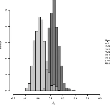
It is important to recognize a key distinction in the behavior of sampling error in genetic eigenvalues compared to any Figure 6 Projection of the observedgmax vector through each of the 10,000 REML-MVN samples ofG(light gray), and the distribution of l1 from 10,000

REML-MVN samples ofG(dark gray). Note how the magnitude of genetic variance from the projection of the single gmaxvector is much smaller than l1 from the same

(13)

particular trait combination. Consider the leading eigenvalue of a given observed Gmatrix, which represents the genetic variance in the trait combinationgmax:As a consequence of the concentration of sampling error in the leading eigen-value, the magnitude of genetic variance ingmax is a combi-nation of that sampling error and the true level of genetic variance. The appropriate null distribution for the eigenvalue ofgmaxis therefore a distribution of leading eigenvalues (as shown above) that all experience the same level of sampling error as the observed eigenvalue. Counterintuitively, this means that the genetic variance in thegmaxtrait combination is tested against the sampling error in random directions in trait space, as in each randomization of a data set the direc-tion of greatest variance will be essentially unique.

From a biological perspective, it may tempting to project the observed traitgmaxvector back through a set ofGmatrices that result from a randomization process, so that the variance in the same trait combination forms the basis of the null distribution. Although this seems to make sense biologically, it will underestimate the amount of sampling error in the observed genetic eigenvalue (Figure 6). This is because the gmaxtrait combination in each realization of a randomization will not capture the concentration of sampling error that resides in the leading eigenvalue.

Testing observed genetic eigenvalues using the TW distribution

The importance of appropriately accounting for sampling error in genetic eigenvalues using the TW distribution is best illustrated by the application of REML-MVN sampling in experimental designs with simulated genetic variance. In our simulated data sets with one genetic dimension, although only a single genetic eigenvalue was simulated in the data, using the 95% confidence intervals from REML-MVN sam-pling would have resulted in the conclusion that a second genetic dimension existed for all three of the experimental designs that were studied. Interpreting the confidence inter-vals in isolation may therefore result in erroneous conclusions regarding the presence of genetic variance (Houle and Meyer 2015; Kingsolver et al. 2015; Wolak and Reid 2016). The overlap of the lower 95% confidence interval with zero will be solely dependent on the power of the experiment: higher (lower) power will result in more (less) spurious genetic eigenvalues detected. Without rescaling these sampling dis-tributions to the TW distribution and using the appropriate critical value of the TW statistic, they do not adequately con-trol for the accumulation of sampling error in the genetic eigenvalues.

In the data simulated to be full rank, factor-analytic mod-eling identified four genetic dimensions that accounted for nonzero levels of variance (Table 2). This is unsurprising given the low expected value of the last eigenvalue of 0.01, and that factor-analytic models are known to be conservative. The TW testing approach, on the other hand, identified all five genetic factors as accounting for significant levels of variance (Table 2). However, the last eigenvalue may not

conform to the TW distribution particularly well. The conse-quence of the downward bias at the tails of the distribution that was observed (Figure 4B) results in an anticonservative hypothesis test when relying on the critical value of the TW distribution. Therefore, the significance of this last genetic dimension identified by TW testing should be interpreted with some caution. At the moment, the TW testing approach will therefore be most appropriate for determining whether leading eigenvalues account for a significant portion of ge-netic variance.

A particularly promising avenue for combining REML-MVN with a TW testing approach may be for very high-dimensional genetic analyses where the convergence of REML would be very unlikely, and where, for example, MCMC is the only viable current approach (Runcie and Mukherjee 2013). If a large number of bivariate genetic analyses are combined to esti-mate aGmatrix (Blowset al.2015), and if the eigenvalues of suchGconform to the TW distribution, it would provide a way to determine the presence of genetic variance in high-dimensional situations without the need for the convergence of high-dimensional models that is currently required.

Acknowledgments

We would like to thank Iain Johnstone, David Houle and Bruce Walsh for helpful comments on the manuscript.

Literature Cited

Aguirre, J. D., M. W. Blows, and D. J. Marshall, 2014 The genetic covariance between life cycle stages separated by metamorpho-sis. Proc. Biol. Sci. 281: 20141091.

Bai, Z., and J. W. Silverstein, 2010 Spectral Analysis of Large Di-mensional Random Matrices, Ed. 2. Springer, New York. Blows, M. W., 2007 A tale of two matrices: multivariate

ap-proaches in evolutionary biology. J. Evol. Biol. 20: 1–8. Blows, M. W., and A. A. Hoffmann, 2005 A reassessment of

ge-netic limits to evolutionary change. Ecology 86: 1371–1384. Blows, M. W., and K. McGuigan, 2015 The distribution of genetic

variance across phenotypic space and the response to selection. Mol. Ecol. 24: 2056_–2072.

Blows, M. W., S. L. Allen, J. M. Collet, S. F. Chenoweth, and K. McGuigan, 2015 The phenome-wide distribution of genetic variance. Am. Nat. 186: 15_–30.

Bryc, K., W. Bryc, and J. W. Silverstein, 2013 Separation of the largest eigenvalues in eigenanalysis of genotype data from dis-crete subpopulations. Theor. Popul. Biol. 89: 34–43.

Chenoweth, S. F., H. D. Rundle, and M. W. Blows, 2010 The contribution of selection and genetic constraints to phenotypic divergence. Am. Nat. 175: 186–196.

Chiani, M., 2014 Distribution of the largest eigenvalue for real wishart and gaussian random matrices and a simple approxima-tion for the tracy–widom distribution. J. Multivariate Anal. 129: 69–81.

Dickerson, G. E., 1955 Genetic slippage in response to selection for multiple objectives. Cold Spring Harb. Symp. Quant. Biol. 20: 213–224.

(14)

Gomulkiewicz, R., and D. Houle, 2009 Demographic and genetic constraints on evolution. Am. Nat. 174: E218–E229.

Hadﬁeld, J. D., 2016 MCMCglmm course notes. Available at: https://cran.r-project.org/web/packages/MCMCglmm/vignettes/ CourseNotes.pdf.

Hadﬁeld, J. D., 2010 MCMC methods for multi-response general-ized linear mixed models: the MCMCglmm R package. J. Stat. Softw. 33: 1–22.

Hadﬁeld, J. D., A. J. Wilson, D. Garant, B. C. Sheldon, and L. E. B. Kruuk, 2010 The misuse of BLUP in ecology and evolution. Am. Nat. 175: 116_–125.

Hazelton, M. L., and L. C. Gurrin, 2003 A note on genetic variance components in mixed models. Genet. Epidemiol. 24: 297_–301. Hill, W. G., and R. Thompson, 1978 Probabilities of non-positive

deﬁnite between-group or genetic covariance matrices. Biomet-rics 34: 429–439.

Hine, E., and M. W. Blows, 2006 Determining the effective di-mensionality of the genetic variance-covariance matrix. Genetics 173: 1135–1144.

Hine, E., K. McGuigan, and M. W. Blows, 2014 Evolutionary con-straints in high-dimensional trait sets. Am. Nat. 184: 119–131. Houle, D., and J. Fierst, 2013 Properties of spontaneous muta-tional variance and covariance for wing size and shape in Dro-sophila melanogaster. Evolution 67: 1116–1130.

Houle, D., and K. Meyer, 2015 Estimating sampling error of evo-lutionary statistics based on genetic covariance matrices using maximum likelihood. J. Evol. Biol. 28: 1542–1549.

Johnstone, I. M., 2001 On the distribution of the largest eigen-value in principal components analysis. Ann. Stat. 29: 295–327. Johnstone, I. M., 2006 High dimensional statistical inference and

random matrices. arXiv math/0611589.

Kingsolver, J. G., N. Heckman, J. Zhang, P. A. Carter, J. L. Knies

et al., 2015 Genetic variation, simplicity, and evolutionary con-straints for function-valued traits. Am. Nat. 185: E166–E181. Kirkpatrick, M., 2009 Patterns of quantitative genetic variation in

multiple dimensions. Genetica 136: 271–284.

Kirkpatrick, M., D. Lofsvold, and M. Bulmer, 1990 Analysis of the inheritance, selection and evolution of growth trajectories. Ge-netics 124: 979–993.

Lande, R., 1979 Quantitative genetic analysis of multivariate evolu-tion, applied to brain: body size allometry. Evolution 33: 402–416. Ma, Z., 2012 Accuracy of the Tracy–Widom limits for the extreme eigenvalues in white Wishart matrices. Bernoulli 18: 322–359. McGuigan, K., J. D. Aguirre, and M. W. Blows, 2015 Simultaneous

estimation of additive and mutational genetic variance in an out-bred population of Drosophila serrata. Genetics 201: 1239–1251. Meyer, K., and D. Houle, 2013 Sampling based approximation of con_ﬁdence intervals for functions of genetic covariance matri-ces. Proc Assoc Advmt Anim Breed Genet 20: 523_–526.

Mezey, J. G., and D. Houle, 2005 The dimensionality of genetic variation for wing shape in Drosophila melanogaster. Evolution 59: 1027–1038.

O’Hara, R. B., J. M. Cano, O. Ovaskainen, C. Teplitsky, and J. S. Alho, 2008 Bayesian approaches in evolutionary quantitative genetics. J. Evol. Biol. 21: 949–957.

Patterson, N., A. L. Price, and D. Reich, 2006 Population structure and eigenanalysis. PLoS Genet. 2: e190.

Pease, C. M., and J. J. Bull, 1988 A critique of methods for mea-suring life history trade-offs. J. Evol. Biol. 1: 293–303. Pitchers, W., J. B. Wolf, T. Tregenza, J. Hunt, and I. Dworkin,

2014 Evolutionary rates for multivariate traits: the role of se-lection and genetic variation. Philos. Trans. R. Soc. Lond. B Biol. Sci. 369: 20130252.

Runcie, D. E., and S. Mukherjee, 2013 Dissecting high-dimensional phenotypes with bayesian sparse factor analysis of genetic covari-ance matrices. Genetics 194: 753–767.

Saccenti, E., A. K. Smilde, J. A. Westerhuis, and M. M. W. B. Hen-driks, 2011 Tracy-Widom statistic for the largest eigenvalue of autoscaled real matrices. J. Chemometr. 25: 644–652.

Schmid, F., and A. Schmidt, 2006 Nonparametric estimation of the coefﬁcient of overlapping—theory and empirical applica-tion. Comput. Stat. Data Anal. 50: 1583–1596.

Sorensen, D., 2008 Developments in statistical analysis in quan-titative genetics. Genetica 136: 319_–332.

Sorensen, D., and D. Gianola, 2010 Likelihood,Bayesian,and

MCMC Methods in Quantitative Genetics. Springer, New

York.

Tracy, C. A., and H. Widom, 1996 On orthogonal and symplectic matrix ensembles. Commun. Math. Phys. 177: 727_–754. Tracy, C. A., and H. Widom, 2009 The distributions of random

matrix theory and their applications, pp. 753_–765 inNew Trends in Mathematical Physics. Springer, New York.

Van Dongen, S., 2006 Prior speciﬁcation in bayesian statistics: three cautionary tales. J. Theor. Biol. 242: 90_–100.

Walsh, B., and M. W. Blows, 2009 Abundant genetic variation + strong selection = multivariate genetic constraints: a geometric view of adaptation. Annu. Rev. Ecol. Evol. Syst. 40: 41–59. Wigner, E. P., 1955 Characteristic vectors of bordered matrices

with inﬁnite dimensions. Ann. Math. 62: 548–564.

Wilson, A. J., D. Réale, M. N. Clements, M. M. Morrissey, E. Postma

et al., 2010 An ecologist’s guide to the animal model. J. Anim. Ecol. 79: 13–26.

Wolak, M. E., and J. M. Reid, 2016 Is pairing with a relative heritable? Estimating female and male genetic contributions to the degree of biparental inbreeding in song sparrows (Melospiza melodia). Am. Nat. 187: 736–752.