Robust predictive control of constrained systems with actuating delay.

University of Windsor University of Windsor

Scholarship at UWindsor

Scholarship at UWindsor

Electronic Theses and Dissertations Theses, Dissertations, and Major Papers

1-1-2007

Robust predictive control of constrained systems with actuating

Robust predictive control of constrained systems with actuating

delay.

delay.

Ali Kebarighotbi University of Windsor

Follow this and additional works at: https://scholar.uwindsor.ca/etd

Recommended Citation Recommended Citation

Kebarighotbi, Ali, "Robust predictive control of constrained systems with actuating delay." (2007). Electronic Theses and Dissertations. 6990.

https://scholar.uwindsor.ca/etd/6990

This online database contains the full-text of PhD dissertations and Masters’ theses of University of Windsor students from 1954 forward. These documents are made available for personal study and research purposes only, in accordance with the Canadian Copyright Act and the Creative Commons license—CC BY-NC-ND (Attribution, Non-Commercial, No Derivative Works). Under this license, works must always be attributed to the copyright holder (original author), cannot be used for any commercial purposes, and may not be altered. Any other use would require the permission of the copyright holder. Students may inquire about withdrawing their dissertation and/or thesis from this database. For additional inquiries, please contact the repository administrator via email

S y stem s w ith A ctu a tin g D elay

b y

A li K ebarighotbi

A Thesis

Submitted to the Faculty of Graduate Studies through Electrical and Computer

Engineering in Partial Fulfillment of the Requirements for the Degree of

Master of Applied Science at the

University of Windsor

Library and Archives Canada

Bibliotheque et Archives Canada

Published Heritage Branch

395 W ellington Street Ottawa ON K1A 0N4 Canada

Your file Votre reference ISBN: 978-0-494-35015-7 Our file Notre reference ISBN: 978-0-494-35015-7

Direction du

Patrimoine de I'edition

395, rue W ellington Ottawa ON K1A 0N4 Canada

NOTICE:

The author has granted a non­ exclusive license allowing Library and Archives Canada to reproduce, publish, archive, preserve, conserve, communicate to the public by

telecommunication or on the Internet, loan, distribute and sell theses

worldwide, for commercial or non­ commercial purposes, in microform, paper, electronic and/or any other formats.

AVIS:

L'auteur a accorde une licence non exclusive permettant a la Bibliotheque et Archives Canada de reproduire, publier, archiver,

sauvegarder, conserver, transmettre au public par telecommunication ou par I'lnternet, preter, distribuer et vendre des theses partout dans le monde, a des fins commerciales ou autres, sur support microforme, papier, electronique et/ou autres formats.

The author retains copyright ownership and moral rights in this thesis. Neither the thesis nor substantial extracts from it may be printed or otherwise reproduced without the author's permission.

L'auteur conserve la propriete du droit d'auteur et des droits moraux qui protege cette these. Ni la these ni des extraits substantiels de celle-ci ne doivent etre imprimes ou autrement reproduits sans son autorisation.

In compliance with the Canadian Privacy Act some supporting forms may have been removed from this thesis.

While these forms may be included in the document page count,

their removal does not represent any loss of content from the thesis.

Conformement a la loi canadienne sur la protection de la vie privee, quelques formulaires secondaires ont ete enleves de cette these.

Bien que ces formulaires aient inclus dans la pagination, il n'y aura aucun contenu manquant.

i*i

All Rights Reserved. No P art of this document may be reproduced, stored or oth­

erwise retained in a retreival system or transm itted in any form, on any medium by

Abstract

Constraints, actuating delay, uncertainties and imperfect state information have many

realizations in the actual applications. These phenomena affect the system analysis

and controller design in th a t care should be taken in designing associated stabilizing

controllers.

This thesis is dedicated to a setting where the constrained control of an input-

delayed linear discrete-time system subject to bounded measurement noise and dis­

turbance input is in question. Using a propagator-based delay compensation strategy

and a set theoretic model predictive control scheme, a robust control synthesis for

such a setting is introduced. More complications arise from the imperfect state infor­

mation.

In this manuscript, a scheme to satisfy the constraints as well as to compensate for

this delay is presented. It is also guaranteed th a t the closed-loop system ’s trajectory

will remain at the vicinity of the origin at the steady state. A number of illustrative

examples verify the theoretic results.

Acknowledgements

I would like to first thank my supervisor, Dr. Xiang Chen whose guidance has been

keeping me on the right research track since the start of my educational career in

Windsor. I would specially like to thank him for his attention to my sometimes spo­

radic thoughts and results on various subjects.

I want also to extend my complements to Dr. Guofeng Zhang with his patience in

helping me to understand the basic ideas of the predictive control and in introducing

me to the fruitful technical resources which were quite effective in helping me quickly

get into the picture of the subject I was researching on.

Needless to say, this work could not be completed without the helpful comments

which I received from my committee members Dr. B. Shahrava and Dr. Z. Hu.

Therefore, I would like to thank them for their contribution to this work.

After all, I would like to thank all the administrative staff in the departm ent of

electrical engineering whose welcoming-ness have made my stay in the University of

Windsor sweet and smooth.

A b stract iv

D ed ica tio n v

A ck n ow led gem en ts vi

List o f F igu res x

List o f A cron ym s xi

List o f S ym bols xii

1 In tro d u ctio n 1

1.1 M o tiv atio n ... 1

1.2 Systems with A ctuating D e la y ... 3

1.3 Constrained Systems and Predictive C o n t r o l ... 5

1.3.1 An Overview ... 5

1.3.2 M ajor MPC s c h e m e s ... 7

1.3.3 Different MPC O p tim iz a tio n s ... 9

1.4 E stim a tio n ... 9

CONTENTS

2 Set Invariance and R o b u st P red ictiv e C ontrol 12

2.1 Model Predictive C o n tro l... 12

2.1.1 Nominal Regulation Problem for M P C ... 13

2.1.2 Dual-mode MPC (DMMPC) - Need for Terminal Cost and Con­ straint ... 15

2.2 Set Invariance and M P C ... 16

2.2.1 Polyhedrons, Polytopes and Their Representations . . . 16

2.2.2 Basic Set-induced O p e r a tio n s ... 18

2.2.3 Set Invariance B a s ic s ... 22

2.2.4 Predicitve Control with Contractive Invariance Constraint . . 25

3 R ob u st P r ed ic tiv e C ontrol w ith A ctu a tin g D elay 29 3.1 Problem F o rm u la tio n ... 29

3.1.1 System sp ecificatio n s... 30

3.1.2 R e q u ire m e n ts ... 31

3.2 Error Bounding E s tim a to r ... 35

3.3 MPC S t r u c t u r e ... 37

3.3.1 Correlation None-observant M P C (C N O M P C )... 37

3.3.2 Correlation Observant MPC (C O M P C )... 47

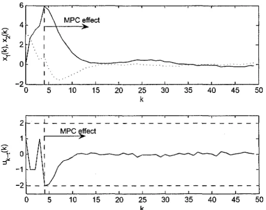
3.4 Illustrative E x a m p le s ... 49

3.4.1 Simulation Based on DP Sets (3 .2 5 )... 50

3.4.2 Simulation Based on DP Sets (3 .3 4 )... 52

4 C on clusions and F uture W ork 55 4.1 C o n trib u tio n s ... 55

4.1.1 Estim ator D e s ig n ... 55

4.1.2 Controller D e s ig n ... 56

4.2 Future W o rk ... 57

R eferences 58

List o f Figures

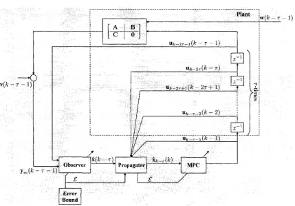
3.1 Problem f o rm u la tio n ... 35

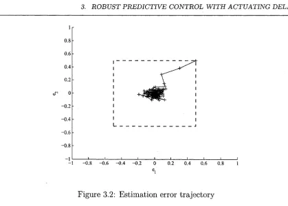
3.2 Estim ation error tra je c to ry ... 50

3.3 Plant states response for Example 3.4.1, r = 3, N = 5... 51

3.4 Invariant sets, propagated state and true future plant state trajectories

pertaining to Example 3.4.1... 51

3.5 Comparing the DP sets computed by (3.25) (dashed style) and (3.34) (dotted

style)... 53

3.6 Plant states response for Example 3.4.2, r = 4, N = 5... 53

3.7 Invariant sets, propagated state and true future plant state trajectories

pertaining to Example 3.4.2... 54

AP Analytical Predictor

AEE Advanced Estim ation Error

AUB Asymptotically Ultimately Bounded

CNOMPC Correlation None-Observant Model Predictive Control COMPC Correlation Observant Model Predictive Control

DAP Discrete Analytical Predictor

DROS Deviation-Robust One-Step

DRS Deviation-Robust Stabilizable

GAP Generalized Analytical Predictor

IMC Internal Model Control

LMI Linear M atrix Inequalities

LPLC Linear Programming with Linear Constraints

MPC Model Predictive Control

MPCCIC Model Predictive Control with Contractive Invariance Constraints

PDI Positively Disturbance Invariant

PD Predicted Deviation

QPLC Quadratic Programming with Linear Constraints

List o f Symbols

The notation used in this thesis is as follows:

Capital Greek and Latin alphabets are used for representing various matrices. Xi

refers to the z-th entry of the vector x or z-th row of m atrix X depending on the con­

text. A zero vector in R n is represented by 0n. Finally, Z + is the set of all positive

integers plus 0.

Notation Definition

© Minkowski addition.

© Minkowski summation operator.

Pontryagin difference operator.

A T Transpose of a m atrix A.

A ° Interior of set A.

A ball with radius e.

R n n-dimensional Euclidean space.

cont(.) Contraction function.

Hausdorff metric.

hull(.) Convex hull of set of points in a vector space.

Pre(.) Preimage of the set as its operand.

Chapter 1

Introduction

1.1

M otivation

The areas of time delay systems and constrained control have long been under inten­

sive investigations. Many advancements have been made in either topic and there is

a myriad of publications pertinent to each subject. However, in actual applications

(e.g. process control and networked control of constrained systems) there are many

situations where the presence of neither of them can be neglected. Unfortunately,

this fact has not received the attention it deserves and the main reason behind this

work is to address this lack.

The time delay and constraints on the system shrink the domain of attraction of

the closed-loop system. Domain of attraction is simply defined as the largest possible

region in the state space in which the closed-loop system is asymptotically stable

[71]. In order to have an effective control, this region should be enlarged as much

as possible. More specifically, effective control demands a method which can ad­

dress the adverse effect of both time delay and constraints on the closed-loop system.

This, hence, motivates one to do an in-depth analysis in both areas and to try to

address their combinatorial problem by means of the available design control tech­

niques. This issue becomes more difficult when besides the stability of the system

some performance specifications are also imposed on the design. These performance

requirements usually appear in the problem setting as new constraints on the behav­

ior of system dynamics. For example, it may be crucial in a design th a t how fast the

closed-loop response of the system is going to be regulated. This kind of performance

specification can be introduced as a set of contractive constraints on the state trajec­

tory of the closed-loop system, for instance.

To make the motif behind the subject more applied, it is also wise to consider the

effect of imperfect state information in control and to account the need for measuring

the output of the plant to reproduce the system states, known as output feedback.

This issue becomes difficult due to various sources of unmeasured uncertainty like, no

perfect model of the plant under control, persistent state disturbances and measure­

ment noise. The effect of these uncertainties makes it impossible to design a controller

able to guarantee the exponential or even asymptotic stability in their original sense

[71]. This makes another motivation which is aimed to design an estim ator which to­

gether with the controller scheme can guarantee the a bounded steady state response

known as ultim ate boundedness [11] of the system.

On the other hand, control of a system suffering from a problem like actuating

delay is effective when the computation of the control does not compromise the hard­

ware infrastructure (e.g. faster CPU and more memory) and is fast enough so th a t

1. INTRODU CTIO N

tools which can be used to tackle this issue.

Given these motivations and requirements for designing a safe estim ator/controller

combination, this thesis concentrates on incorporating the effect of delay and uncer­

tainties in design of a controller which beside guaranteeing stability guarantees th at

the constraints will not be violated and compensates for the actuating delay after a

short interval as if no delay is present in the control input.

The rest of this chapter is devoted to give the reader a background on the works

already done for the tim e delay systems and constrained control. The intention is to

highlight the motivations more specific to each field as well as to their overlap. A

note on the thesis structure is also included at the end.

1.2

S ystem s w ith A ctuatin g D elay

The control of time delay systems has been the hot spot for the last years and has

already received a lot of attention. The motivation behind this push first came from

the process industry since there were many examples of the delay systems which re­

quired a better control than the conventional memoryless P I controllers (e.g. heat

exchangers and feeding/exhausting systems in the process plants). As a result of such

motivation many theoretical advancements have been made during the last decades.

See for example, [35, 78, 88] for comprehensive survey on the recent results in this

realm. Interesting discussions on the controllability of actuating delay systems can be

found in [44, 45, 46] for both continuous and discrete-time systems. For some books

on the subject reader may be referred to [34, 48, 57, 58, 70]. Unfortunately, except

for [70] which has a dedicated part for actuating delay most of the material available

is on the systems with state delays, though the control of systems with actuating is

no less challenging.

The developments of the theoretical ground for control of the systems with ac­

tuating delay has tracked two somehow independent ways for continuous-time and

discrete-time systems but started within the same tim e frame. The credit for discus­

sion in the continuous-time domain goes to [2, 54, 59] wherein authors advocate the

use of propagator based controller (e.g. a controller which works on the future states

of the system rather than the present states) to enlarge the domain of attraction of

the resulting closed-loop dynamic system. Their approach is then tailored for robust­

ness against uncertainties in many publications (e.g. see [47]) which usually consider

a robust analysis for the systems with state feedback. Although not as fruitful as

propagator-based control, some efforts have also been made on tailoring the existing

non-delay methods or memoryless feedback schemes [20, 85, 91] in order to achieve

a degree of robustness. However, it has been shown via simple analysis [80] th a t the

memoryless controllers are far inferior to the propagated-based schemes.

By the advent of the digital control, some developments in the discrete-time sys­

tems was needed. Many propagator-based theories has been developed for the nomi­

nal systems. Smith predictor which has attracted so much attention in the industry

was first introduced by [86]. In the nominal sense it could compensate for the ac­

tuating delay very easily. Due to the poor stability of smith predictor design other

schemes addressing actuating delay have emerged. See for example, [27, 28, 29] for

internal model control (IMC), [23, 67] for analytical and discrete analytical predictor

(A P/D A P) schemes and generalized analytical predictor (GAP) [89, 90]. IMC also

has got some attention in the industry due to better steady state performance as op­

posed to Smith predictor. However, because it utilizes the inverse of the plant model,

the model of the plant should exactly be known. Also demerits of the Smith predictor

1. INTRODU CTIO N

AP, DAP, and GAP ameliorated these demerits and have shown better steady state

response and better robustness to known uncertainties, however, they also fall short

in case of unmeasured perturbations. To avoid scattered discussion an in-depth anal­

ysis cannot be given on these schemes here. A basic comparison of these schemes

is given in [90] where it can be concluded th a t all the schemes fall short when it

comes to the systems with uncertainties where f unmeasured disturbance or modeling

error is present. Later, some researchers have attem pted to modify these schemes in

order to use them for the unstable systems [3, 66, 64, 87], though not with big success.

All in all, the result of the researches done to date justifies the fact th a t more or

less there is not much one can do to control of the input-delayed systems when the

they suffers from unknown or unmeasured uncertainties either in the form of modeling

error or in the form of exogenous disturbance and noise. By using a propagator which

is in a way related to DAP and the work done in [2], it will be shown in later chapters

th a t the effect of this issue strains the controller design and certain cares should be

taken while designing a controller to stabilize the general systems with actuating

delay.

1.3

C onstrained System s and P red ictive Control

1.3.1 A n O verview

In terms of finding applications in industry, theories developed for the constrained

systems come in the second position after the regular linear system theories. This

is due to the fact th a t simply all the controlled systems have either implicitly or

explicitly constraints on their input or states. In many applications like ship rudder

control or compressor systems not attending to the existence of such constraints is

The constrained control via schemes other than predictive control is not common.

However, some researches have been done in this direction. In [38] a procedure is

presented in order to maximize the attractive region of the input-constrained closed-

loop system with linear feedback. Using linear m atrix inequalities (LMI) [13] a way

to determine the maximal domain of attraction of linear systems, albeit in the form

of an ellipsoid, is introduced. Differently, [75] has used the invariance set theory in

order to characterize the domain of attraction in the form of a polytope. Each taken

approach assumed linear state feedback law. This is because nonlinear control syn­

thesis for such systems in optimal scheme requires finding a robust control lyapunov

function (RCLF) [26] which is not an easy task for general nonlinear systems in most

of the cases. Moreover, the design of the proposed linear law is done offline removing

the chance to change it according to the changing online conditions.

On the other side of the spectrum comes the MPC which is related to the op­

timal control concept and is tailored mainly to consider constraints on the system’s

input an d /o r states. It is a recursive methodology wherein at each time instant an

optimization is performed over a future control input trajectory rather than a con­

trol input alone. Implementation is done by applying only the first entry of such a

trajectory to the plant. MPC removes the shortcomings of the other constrained con­

trol approaches by adopting a time varying control law which can adapt to condition

changes and introducing variations with nonlinear law which are easy to implement

and can have an immense effect in enlarging the domain of attraction of the closed-

loop system [81]. These capabilities has turned MPC into a popular control approach

with over 2000 reported applications [61]. Also it is known as the only advanced

method with significant impact on the industry [56]. This is no surprise by knowing

1. INTRODUCTION

For the cogency of discussion further notes on the origin of MPC is om itted here. A

comprehensive note on MPC history can be found in [56].

1.3.2

M ajor M P C schem es

In this section the aim is to discuss the major MPC schemes which have found good

merits in terms of a combination of robustness, optimality, and computational inten­

sity. For comprehensive notes on various types of MPC schemes to date reader may

consult several surveys and books on the model predictive control [6, 56, 68, 63, 77].

The nonlinear MPC schemes are discussed in [61, 63, 72], Also, industry-oriented

discussions can be found in [73, 74],

The MPC scheme which was first used in the industry had a finite horizon l .

However, It is proven th a t finite horizon scheme falls short in stabilization of the

systems [56]. As a remedy to this problem a dual mode MPC (DMMPC) was then

introduced. In this scheme a terminal cost and a terminal constraint have been added

to the finite horizon MPC in order to emulate an infinite horizon problem. The idea

of using a term inal cost and constraint at once to guarantee nominal feasibility as well

as stability was first introduced in [41], where the terminal constraint was chosen to

be the origin, i.e. T — {0}. However, this constraint reduces the size of the feasible

set and could result in numerical convergence problems in the optimization, especially

when working w ith nonlinear models [61]. Also it could not be extended to the case

of systems with uncertainties.

One of the most popular MPC methods for guaranteeing robust stability is to

choose an invariant term inal set [65]. Such a set has a feature th a t every state trajec­

tory starting inside this set will remain in its interior for unlimited time. By choosing

1 Discussions on finite and infinite horizon problems can be found in Chapter 2.

the terminal constraint to be such a set, rather than the origin, the size of the feasi­

ble region of the MPC optimization for a given horizon N is increased and most of

the numerical convergence problems are addressed. After introduction of this noble

approach to the academia almost all the robust MPC schemes proposed were in a

way a subsidiary to it. M ajor schemes which have found considerable attentions are

[5, 18, 51]. Among these schemes model predictive control with contractive invariance

constraint (MPCCIC) [18] is chosen and extended in this thesis resulting in a whole

new method. This scheme makes the grounding of the main discussion of the thesis

which can be found later in Section 3.3. It is based on set invariance theory [12] and

involves com putation of problem-relevant invariant sets or attractive regions prior to

doing any online optimization. This has the effect of less online computation which

is amicable for actuating delay problem.

It is also im portant to point out th at using this approach one can easily take the

state estimation error and actuating delay into the consideration. This then can be

seen as a remedy to problem of output feedback in MPC which has not lent itself to

full disclosure yet. In fact, there are only few useful papers published on this issue

[4, 55, 62, 83] which as a result make this area remain fairly open to new investiga­

tions. The cause of this issue is the strict dependence of MPC predictions on the

current system state. Therefore, any error in the state measurement yields predic­

tions which are not close to the actual plant state trajectory in future. An adequately

updated survey on the output feedback MPC can be found in [25].

There are other DMMPC schemes which have considered the delay in the system.

The major work is done in [51] which spawned a series of schemes based on LMIs

[39, 40, 80]. However, LMI approach has the shortcoming in th a t it is not clear how to

1. INTRODUCTION

rapidly with number of the states and amount of delay in the system which renders

it an online-computationally demanding scheme [56].

1.3.3 D ifferent M P C O ptim izations

All the MPC schemes which have found considerable attention in the industry assume

either linear or quadratic constraints for the processes under control. The reason is

th a t using nonlinear constraints can yield to non-convex an d /o r nonlinear optimiza­

tion problems which then put the computation resources under pressure. Common

optimizations involve quadratic programming with linear constraints (QPLC) and

linear programming with linear constraints (LPLC). However, there are instances of

successful schemes using quadratic programming with quadratic constraints (QPQC)

[52] albeit at the expense of heavier but tolerable computations. Since quadratic

constraints, usually in terms of ellipsoids, can fall short in tightly approximating the

actual constraints on the system, theoretical developments in this thesis has been

grounded on linear constraints. Furthermore, the scheme proposed in this thesis is

intended to compensate for delay and base a procedure to address faster applications

like networked control [92]. Hence, using the quadratic constraints is not advocated.

1.4

E stim ation

There are various estim ation/reachability analysis technics using for examples ellip­

soids [9, 16, 53, 82], zonotopes [1, 31] and parallelotopes [17] to define a guaranteed

state estimation. However, each of these approaches has shortcomings when compared

to the polytopic approach taken here. For example, each step in the estimation by

ellipsoids requires outer-approximation of the resulting estimation error bound which

is detrimental to precision of the analysis. Zonotopes and parallelotopes are special

polytopes and this speciality makes them not as flexible as the general polytopes in

estimation of an arbitrary region in the space. A brief comparison is given in [76].

It is known for a while th a t coupling an stable state estim ator and a nominally

exponentially stable M PC scheme will result in asymptotic closed-loop stability of the

whole system given the disturbances and noises are decaying overtime [84]. However,

when the problem deals with the persistent uncertainties in the form of unmeasured

disturbance input, measurement noise, finding a control scheme to guarantee asymp­

totic stability is not possible. The reason is th a t when the perturbations are persistent

using an stable estim ator can only guarantee a bound on the state estimation error

and the problem of coupling of such an estim ator with a nominally exponentially

stable MPC scheme does not guarantee even the asymptotically ultim ately bounded

(AUB) stability2. However, it is shown in [60] th a t by applying invariance theorem

one can achieve the AUB stability of the closed-loop response.

The idea of set invariance for designing an estim ator first published in [24] where

a method to define a polytopic bound on the estimation error is proposed for the

systems with disturbance input. In this thesis, the idea in [24] is extended to the case

where the measurements are contaminated by persistent but polytopically bounded

noise.

1.5

Structure o f Thesis

This thesis is organized as follows:

C hapter 2: S et Invariance and R ob u st P r ed ic tiv e C ontrol

In Section 2.1, a preliminary definition on the MPC is given in both nominal case and

1. INTRODU CTIO N

general dual mode scheme. Section 2.2 is dedicated to give preliminaries regarding

the poly topic objects and their representations. A group of set valued operations and

tools is also defined and characterized in this section. In particular, Section 2.2.3 is

devoted to the discussion on the basics of the set invariance in control. The way to

design and implement the invariance sets under time-invariant linear feedback law as

well as time-varying controller schemes is also discussed ifi this section. The final sec­

tion of Chapter 2 regards to the MPCCIC scheme since it is needed for understanding

the materials given in Chapter 3.

C hapter 3: R o b u st P r ed ic tiv e C ontrol w ith A ctu a tin g D ela y

The main contribution of this work is squeezed in this chapter. Chapter 3 begins with

the analysis and design of a error-bounding state estim ator which is a extension to

the work done [24]. It also deals with introducing a linear set propagator which plays

an im portant role in compensating for the actuating delay as well as in enlarging

the domain of attraction of the resulting closed-loop system. The discussion on the

proposed MPC approach is given in section 3.3. This includes the notes on designing

various invariant sets like terminal constraint and a new feasibility and stability guar­

anteeing constraint set for the proposed MPC model. Section 3.4 is then intended

to verify the theoretics developed in the previous sections of this chapter via a set of

illustrative examples.

C hapter 4: C on clu sion s and future work

This chapter summarizes the contributions made by this thesis and outlines directions

for future research.

Set Invariance and Robust

Predictive Control

In this chapter, first an overview of the model predicitve control methodology is given.

The basic conceptual definitions are explained and different tools needed to operate on

sets are characterized. General idea behind the set invariance theory and its relation

to MPC is also discussed. In particular, The MPCCIC scheme is also introduced to

provide prerequisites to help assimilate the discussion in the main part of this thesis.

2.1

M odel P redictive Control

Assume a case in which no disturbance is present and exact state information is

available for control-related computations. Let a system dynamics be summarized as

the following:

2. SET INVARIANCE AND R O B U ST PREDICTIVE CONTROL

where k is the tim e step, x € R n, u 6 R m, and w e R " and / : R n x R m x R n —> R n

is general time-invariant continuous function of state x, input u and the disturbance

input w. It is also assumed th a t /(•, •, •) possesses a fixed point at origin, i.e. 0n =

/( 0 n, 0m, 0„). The following set memberships are also held

x (E X 3 0n, (2'2)

u e U 3 0m, (2.3)

w 6 W 3 On. (2.4)

where X is a generic set and U is compact. Model predictive control is a scheme in

which a nominal copy of plant model (i.e. when w = 0n) known as internal model is

used to predict the future states and inputs of the plant. In this section, a brief dis­

cussion is dedicated to the MPC schemes defined for the system (2.1) under different

conditions.

2.1.1

N om in al R egu lation P roblem for M P C

Consider the dynamics (2.1) where it is assumed th a t w(k) = Ora,VA: e Z + . The

nominal MPC problem can be described by the following procedure:

• At each instant k find the solution to the following constrained optimization

problem:

N - l

u opt = min L( x ( k + i\k), u(k + i\k)), (2.5a)

i=0

u = [u(k\k)T , u(k + 1|A;)T, . . . , u(k + N — l|fc)T]T, (2.5b)

subject to

x(k\k) = x(k), (2.5c)

x( k + i + l\k) = f ( x ( k + i\ k), u( k + i\k),On), (2.5d)

x ( k + i \ k ) e X , i = 0 , . . . , iV — 1, (2.5e)

u{k + i\k) G U, i = 0 , . . . , iV — 1, (2.5f)

• Set the actual input u(k) = u(k\k) and repeat the optimization with updated

d ata at next sampling instance.

In the above optimization x( k + i\k), u(k + i\k), i = 0 , . . . , N — 1 are the M PC’s

predicted state and predicted control input respectively. They are defined as predicted

state and predicted input of the system for time step k + i which are evaluated based

on the state information at time k, i.e. x(k). (2.5d) is the M PC ’s internal model

used to do the predictions. L(. , .) is called stage cost function which is a continuous,

non-negative and tim e invariant function defined on X x U.

It is known [56] th a t due to finite horizon nature of the problem (i.e. when

N < oo), optimization (2.5) cannot guarantee feasibility nor stability of closedloop

dynamics in any sense. The following general scheme is then introduced to get over

2. SET INVARIANCE A ND R O B U ST PREDICTIVE CONTROL

2.1.2

D u al-m od e M P C (D M M P C ) - N eed for Term inal Cost

and C onstraint

Considering (2.1), a generic DMMPC optimization can be represented by

N - l

u opt — min F( x ( k + N\ k)) + L( x( k + i\k), u(k + i\k)), (2.6a)

i=0

u = [u(k\k)T , u(k + 1|k)T, . . . , u(k + N — 1|&;)T]T, (2.6b)

subject to

x(k\k) — x(k), (2.6c)

x( k + i + l\k) = f ( x ( k + i\k), u(k + i\k), 0n), (2.6d)

x( k + i\k) € X , i — 0 , . . . , iV — I, (2.6e)

u(k + i \ k ) e U , i = 0 , . . . , N - I, (2.6f)

u(k + i\k) = g(x(k + i\k)) € U, i > N , (2.6g)

x( k + i\k) 6 T C X , i > N, (2.6h)

where F(.) is the terminal cost which is a non-negative, time invariant and continuous

function on X . g(.) is a time invariant function on X which defines a time-invariant

state feedback law inside the set T . T itself is called the terminal constraint.

Remark 2.1: The reason for naming this scheme as dual-mode is caused by the

fact th at for the predicted control inputs with indices higher th a t th a t of horizon

N, control law switches from MPC law to a fixed control law defined by g(.). In the

simplest case g(.) can be a linear state feedback law which is will be discussed later

in this chapter.

Remark 2.2: It had been known (e.g. see [10]) for quite some time th at using

Bellman’s principle of optimality one can use the problem (2.5) with infinite horizon,

i.e. setting N = oo. However, it was not known how to handle constraints with infinite

horizon since it makes (2.5) an infinte-dimensional problem for which a solution can

not be conceived. DMMPC has solved this problem by doing the optimization over

an iV-tuple trajectory with m atrix representation (2.6b) and relegating the rest of

the problem to time-invariant control law (2.6g) for which a term inal cost F(-) can

be defined.

2.2

Set Invariance and M PC

Invariance concept in control has been considered relatively early in modern control

literature (e.g. see [22]) and is proven as a tool both in analysis and synthesis of

control sysytems [12]. This section is dedicated to relation of set invariance and MPC

methodology.

2.2.1

P olyh ed ron s, P olytop es and Their R ep resen tation s

Definition 2.1 (Closed Half-space): Consider n-dimensional Euclidean space R n.

Associated with any constant vector 7r G R n, n A 0n and a constant 9 G R., there is a

Closed Half-space defined by

H{ir, 6) = { x e R n|7rTx < 9}. (2.7)

Definition 2.2 (Polyhedron): A convex set, A C R n, is called a polyhedron if it

can be represented by a finite intersection of closed half-spaces.

W'ha

A = P | 9i), TCiG R n, 9i G R

i —1

where ri/ia is the number of half-spaces involved.

Using (2.7), a polyhedron can be represented by its half-space representation of

the form

2. SE T INVARIANCE AND R O B U ST PREDICTIVE CONTROL

where II G R n'iaXn and 0 G In particular, for a polyhedron A containing the

origin in its interior A°, a representation (2.8) exists where > 0, i = 1, . . . , n /la[50].

Definition 2.3 (Extreme Point): Consider a convex set A G R n. A point a is an

extreme point of A if and only if

a G A : $ai, a,2 G A, $ A G (0, 1) such th a t a = (1 — A)ai + Aa2.

Intuitively extreme points of a convex set are the corners or vertices of th a t set. The

set of all extreme points of A is called extreme set of A .

Definition 2.4 (Convex Hull): Consider a set of points A = {a, G R n, i =

1, . . . , n}. The convex hull of A is a set A represented by

n n

A — hull(A) = {a G R n|3Ct = {a^, i = 1 , . . . , n : on > 0, a* = 1} and a ~ eqaj}

t=1 i—1

(2.9)

and is intuitively the minimal convex envelope containing all points in A.

Theorem 2.1: [79], Consider a convex set A with a countable extreme set A —

{a,i G A , i — 1 , . . . , n va}. Let also A = {a* G A , i = 1 , . . . , n } be arbitrary. Then A

has the minimum number of points such th a t hull(A) = A if and only if A = A.

Proposition 2.1: Let A be a polyhedron with extreme set A = {a;, i = 1, . . . , n va}.

Then A has also a convex hull representation of the form

A = hull(A) = hull({oi,z = 1, . . . ,n m }). (2.10)

Remark 2.3: Representations (2.8) and (2.10) are interchangeable. However, as

the dimension and the number of half-spaces grows finding all vertices of the polyhe­

dron which involves a mix of search and linear programming (LP) can become quite

demanding. The same is also true for finding a numerically robust algorithm which

can compute the convex hull of a large number of points [21].

Definition 2.5: A set A G R n is said to be bounded if and only if there exists a

constant r > 0 such th a t A C 93r , where W = {x G R n : ||x|| < r } 1.

Definition 2.6 (Polytope): A bounded polyhedron is called a polytope.

Definition 2.7: A polytope A is said to be symmetric if and only if Va G A , — a G

A . Briefly shown, A is symmetric if A = —A.

Remark 2.4: In order to have a compact and unified representation, a notation

K n is adopted in this thesis to define all compact and convex sets in R n. Notice th at

in this sense polytopes in R n are members of K n.

2.2.2

B asic S et-in d uced O perations

Definition 2.8: Consider a polyhedron A C R n with half-space representation

(2.8). Then affine translation of A with respect to the translation vector v G R Tl is a

set B C R n and is defined by

B = v + A = { b e R n|II& < 0 + Uv}.

Definition 2.9: Given two polyhedrons

A = { a c

Rn|n xa

B

Rn|II26 < 0 2},

their intersection is a set C C

Rn

(2.11)

C = A n B c g R"

Ill

0 X C <

n 2_ 0 2_

Remark 2.5: The m atrix concatenation above may yield redundant inequalities.

These inequalities may strain the computations involving these sets since they cause

redundant computations. To tackle this problem some methods already are intro­

2. SET INVARIANCE A N D R O B U ST PREDICTIVE CONTROL

Definition 2.10: Let A G Kn be a polytope and T : R n —> R m be a linear transfor­

mation. The linear transformation of A is a set B C R m with the following definition

B = T ( A ) = { b e R m|b = T(a), Va G

A}.

When the transform ation is written in the form of a m atrix in R mxn, m > n, two

situations might arise which are discussed by the following theorems.

Theorem 2.2 (T G R mxm is invertible [8, 42]): Assuming A possesses the repre­

sentation (2.8), the linear transformation of A can be w ritten as

B = T A = { b e

Rn|nT_16

0}.

Theorem 2.3 (T G R mxn, m > n [42, 69]): Let r = rank(T). Then

B = T A = { b c R m|

T±6

nTjft

0}

where rows of T± G R(m~r)xm form a basis for subspace of R,m which is orthogonal to

the subspace spanned by columns of T and Tj is any m atrix with property T jT = Im.

A more elaborated account on these theorems as well as their proofs can be found

in [42]. As a general alternative to Theorems 2.2 and 2.3, the following theorem

can be used to address the problem of linear transformation. However, according to

Remark 2.3, this may cause heavy computations when the number of vertices is large.

Theorem 2.4: [79] Let A G K n be a polytope. Assume A — vert

(.4) =

Then the set B = T(A ) is a subset of K m with the set of vertices B = {bj , j =

1. . . . ,n vb} such th at

n vb < n va and Vbj G B , 3fo G A :bj = Taj.

Theorem 2.5: [79] Consider a countable set of points A in R n. Let also B be a

set of points in R n such th at A C B . Then hull(A) C hull(B).

Definition 2.11: Consider a polytope A G Kn and a linear m atrix transformation

T : R” —>• R m. Then, pre-image of A with respect to T is defined as

Pre(M) = { x € Rn|Tx G A }.

Definition 2.12 (Support Function [36, 50, 79]): The support function of a set

d c R 11 calculated at a given direction r; G R n is defined by

hA (rj) = sup(7/Ta).

Furthermore, if A is a polytope with representations (2.8) and (2.10), then

Definition 2.13 (Minkowski Addition [36]): Consider A and B as two generic sets

in an Euclidean space. The Minkowski addition of the two sets is described by

C = A © B = {c = a + b : a G A ,b G B},

The notation will also be used in order to show the sum operator for this type

of addition.

Lemma 2.6: [33] W hen the operands A and B in (2.14) are polyhedrons, their

Minkowski addition can be computed as per following,

^Aiv) = niax(?7Ta), aG vert(M ). (2.13)

a

(2.14)

2. SE T INVARIANCE AND R O B U ST PREDICTIVE CONTROL

Remark 2.6: Lemma 2.6 suggests th a t Minkowski addition can be done through

finding the vertices of each operand and then, finding all combinations of addition of

their vertices and taking the hull of the resulting combinations.

The following theorem characterize the relation between support function of the

sets and their Minkowski addition.

Theorem 2.7: [79] Let A and B be two sets with their Minkowski addition defined

in (2.14). For any direction p G Rn, we have

hc(rj) > hA (rj) + hB(r]).

Definition 2.14 (Pontryagin Difference [36]): Given two generic sets 4 c R n and

B G K n , the Pontryagin difference or shortly p-difference between A and B is defined

by

C = A ~ B = {c G R n |c + B C A }

= r v - » - (2'i6 >

beB

Theorem 2.8: [50] Let A and B be such th a t their p-difference (2.16) is defined.

For any direction 77 G R n, we have

h c ( v )

<

) - M

7?)-Lemma 2.9: [50] Let A and B be sets in Euclidean space such th a t A B ^ t b .

Let B — B\ © B2, then

A ~ B = {A ~ Bi) ~ B2. (2.17)

The following lemma shed light on the way with which the p-difference can be

computed for polytopes.

Lemma 2.10: [50] Suppose A C R n is a polyhedron with representation (2.8), and

assume B e K" is a poly tope for which hs{TTi),i = 1, . . . , n ha, then

A ~ B = {c G R n|7rfc < Oi - hB(ni), * = 1, • • •, ^ a } (2.18)

Definition 2.15 (Hausdorff Metric [14]): The distance between two compact sets

M, B C R n can be discribed by Hausdorff metric which is defined as

dh(A, B) = inf{e > 0|M C Bt and B C A }

where A e and Bt denote the union of all closed balls of radius e centered at points of

A and B respectively.

Proposition 2.2: Let <B t be a closed ball with radius e centred at origin. Then,

according to the definition 2.13, in defintion 2.15 we have

A t = A® <B€ and B t = B @ W .

2.2.3

Set Invariance B asics

The following discussion grounds the idea behind the set invariance concept for linear

discrete-time systems. The concepts given here will be extended in Chapter 3 to

address the main contribution of this thesis.

Consider the following constrained linear discrete-time system

x( k + 1) = Ax(k) + Bu i k ) 4- w(k),

u ( k) = h(x(k)),

y ( k) = Cx(k). (2.19)

2. SE T INVARIANCE AND R O B U ST PRE D ICTIV E CONTROL

realizaton of the disturbance input. Function h : R ra —> R m is the feedback control

law on the perfect state information x and is assumed to be continuous. y{k) G Rp

is the system output. Moreover, it is assumed th a t the matrices A, B, and C have

compatible dimensions. The system is subject to the following constraints,

x e X , on e X (2.20)

u e u , om e u , (2.21)

where X is assumed to be a polyhedron in R n and U G K n is assumed to be a

polytope. Furthermore, no information is assumed on the disturbance input w(k)

except for a polytopic set membership

w e w , 0n € W . (2.22)

Remark 2.7: Compared to (2.1), the state evolution in (2.19) can be found by

setting f ( x ( k ) , u ( k ) , w ( k ) ) = Ax(k) + Bu( k) + w(k). Also here, A is a polyhedron

and U is a polytope which results in a more restricted condition.

For the system (2.19), basic invariant sets under different control laws are discussed

in the sequel. A more general discussion for the case of nonlinear feedback law, h(-),

can be found in [42, 43].

Invariant S ets under Linear T im e-invariant S ta te Feedback, h(x) = K x

Let in (2.19) the control law be defined by,

u(k) = h(x) = Kx ( k ) , (2.23)

then

x( k + l) = {A + B K ) x { k ) + w { k ) , (2.24)

where it is assumed th a t K is such th at the m atrix $ = A + B K is stable, i.e. all its

eigenvalues lie inside the unit circle.

Definition 2.16 (Input Admissible Set [43]): For the system (2.19), a set X ad Q X

is called input admissible under the linear state feedback law (2.23) if and only if

X ad = {x : x e X , K x G U}. (2.25)

Definition 2.17 (Positively Disturbance Invariant(PDI) Set [49, 50]): For the sys­

tem (2.19), a set T is called PDI under linear time-invariant state feedback if and

only if for a tim e step k0, we have

Vx(fc0) € T and Vw(k) G W, x(k) G T and u(k) = K x ( k ) G U. Vk > k0. (2.26)

Proposition 2.3: If T is a PDI set then by the condition (2.26) we have T C X ad.

Proposition 2.4: T is a PDI set if the following condition is satisfied:

(A + B K ) T C T ~ W , T C X ad. (2.27)

Remark 2.8: PDI set can be defined for any general nonlinear but time-invariant

feedback law [42]. However, in this thesis PDI set alludes to linear state feedback law

(2.23).

Invariant S ets under A ffine Feedback, h(x) — K x + q

Consider (2.19) with the control law defined by

u(k) = K x ( k) + q(k), (2.28)

where q(k) is a residual computed via a control law other than state feedback so as

to give more flexibility in controlling (2.19). Then, (2.19), can be w ritten as

x( k + l) = (A + B K ) x ( k ) + B q ( k ) + w ( k ) , k > 0. (2.29)

Definition 2.18 (Robustly Stabilizable Set [7, 43]): Assume (2.29) admits a PDI

2. S E T INVARIANCE AND R O B U ST PREDICTIVE CONTROL

X , is called M-step robustly stabilizable set for (2.29) if and only if it contains all

states in X for which there exists a time-varying feedback control law (2.28) which

produces an input trajectory {u(k) — K x ( k) + q(k)}^lo1 which satisfies the input

constraint (2.21) and drives the system state to T in M steps or less, while keeping

the evolution (2.29) inside the state constraint X. M athematically speaking, this is

equivalent to say

S M(X, T ) = {z(0) € R"|3{u(fc) = Kx ( k ) + q(k) e U}%r0\ 3 N < M :

{ x{k) e X } ^ - Q\{ x { k ) € T}%LN ,V{w(k) € W j j l o 1} 'I2-30)

Proposition 2.5: The following condition is true for stabilizable sets. For any

positive integer N ,

S N { X,T ) D Sn_i( X , T ) D . .. D S x{ X , T ) D S 0( X , T ) = T .

In this m anuscript, the arguments ( X , T ) may be excluded for brevity whenever

it does not cause confusion.

2.2.4

P red icitv e C ontrol w ith C ontractive Invariance Con­

straint

MPCCIC scheme is a variant of DMMPC. Because the controller scheme which is

going to be proposed in this thesis is infact inspired by model predicitve control with

contractive invariance constraint (MPCCIC) [18], here a brief section is dedicated to

its background. Beforehand, the following definition is in order.

Definition 2.19 (Asymptotically Ultimately Bounded Stability [11, 60]): Consider

a system resulting from (2.19) by omitting constraints (2.20) and (2.21) and u = 0.

This system is called asymptotically ultimately bounded(AUB) if the system evolves

asymptotically to a bounded set, i.e. there are finite constants /?, 7 > 0 such th at

the following condition is satisfied.

Va £ (0,7), 3k* > 0 : ||x(0)|| < a => ||a:(fc)|| < /3, VA: > k*

where ||.|| can be any vector norm.

To give a definition for the case in which u ^ O and constraints (2.20) and (2.21)

are present the following proposition is given.

Definition 2.20: The system (2.19) is said to be AUB stabilizable if there exists

an initial state s(0) £ X and an infinite input trajectory {u{k) £ which

can satisfy the following conditions disregarding all possible disturbance trajectories

{w{k) £ W}£°=0:

(i) x ( k) £ X , k = 0 , . . . , 0 0.

(ii) 3k* > 0 such th a t for all k > k*, ||:z(/c)|| < (3, ft > 0 is such th a t ||x|| < fi =7

x C X.

The set of all initial states which admit an admissible input trajectory to guarantee

these two conditions is called AUB stabilizable set.

M P C C IC d efin ition

Here, a variant of MPC which is then extended in this thesis to form the main

contribution is discussed. If the quadratic stage cost and term inal cost is considered

and an affine control law (2.28) is assumed, the MPCCIC scheme at time step k can

be implemented by a quadratic programming with linear constraints (QPLC) over a

2. S E T INVARIANCE AND R O B U ST PREDICTIVE CONTROL

• Having the perfect state information x(k), solve

qop = arg n u n J (N ),

, J V - l

J ( N ) — < x T (k + N \ k ) P x ( k + N\ k) + ^ [xT (k + i \ k)Qx(k + i\k)+

^ i=0

qT (k + i \k)Rq(k + i\k)]

j,

q = [qT(k\k), . . . , qT (k + N - l\k)]T , (2.31b)

subject to

x(k\k) = x(k), (2.31c)

x( k + i + l\k) = A x ( k + i\k) + B u (k + i\k), (2.31d)

u(k + i\k) = K x ( k + i\k) + q(k + i \ k ) e U , (2.31e)

x ( k + i \ k ) e X , (2.31f)

x( k + N\ k) G T , or q(k + i\k) = 0m, i > N , (2-31g)

x( k + l\k) e Scon C X, (2.31h)

P > 0, Q > 0, R > 0, (2.31i)

• P u t u(k) — K x ( k) + q(k\k) and repeat the optimization at th next time step.

In this procedure,q is the m atrix representation of the predicted auxiliary input tra­

jectory. T is the term inal constraint and assumed to be PDI under state feedback

(2.23). (2.31i) simply means matrices P and Q are positively semidefinite and R

is assumed positively definite. This assures th a t the stage cost and cost satisfy the

reuirements discussed in Section 2.1.1. S con is called contractive invariance constraint

which involves a contraction of a proper stabilizable set defined in (2.30) and is cal­

culated by the following algorithm:

Algorithm 2.1: At each tim e instant k, considering x(k) as the true plant state

1. Check if x(k) G <Syv, where N is considered the smallest integer which makes

this condition true.

2. Impose an constraint on MPC which makes x( k + 1) G <Sjv-i true. By (2.29)

this can be w ritten in terms of the MPC predicted state (2.31d) which is the

same as (2.29) but with no disturbances w(k) G W,he.

x{k -p l|fc) G <Sjv-i ~ W x{k -\-1) G <Sjv—i ^ S con — <Sjv_i ~ W. (2.32)

Remark 2.9: AUB stability of the MPCCIC scheme comes from the fact th a t each

stabilizable set Si, i = 0 , . . . , N — 1 satisfied the AUB condition in Proposition 2.20.

Chapter 3

Robust Predictive Control with

Actuating Delay

This chapter embraces the major contribution and results of this thesis. It starts

with the problem formulation. Then using a combination of disturbance invariance

concept [24] and the set-membership membership estimation [82] an estimator is

designed which guarantees a polytopic bound on the estimation error. Later, this

bound is used in designing an output feedback MPC scheme which together with the

proposed estim ator guarantees the AUB stability. More improvements are given by

considering the observer dynamics and a correlation between the uncertainties. The

proposed scheme also compensates for the delay in the control input.

3.1

P roblem Form ulation

First, let us introduce two new notations.

Definition 3.1: Consider a polytope A G R n and a trajectory {a(k) G A }^L0.

Then a time-stamped polytope A( k) G R n is a set such th a t Yk G Z + :

• It is shape-wise time-invariant, i.e. A( k) = A.

• Only a(k) G A(k).

Definition 3.2: Consider a trajectory {u(&)}fcL0. Then, a polytope denoted by

A t (k) with k and t as integers and t < fc, refers to a polytope computed at time t

such th a t it defines a set at time k: At{k) 3 a(k).

3.1.1

S ystem specifications

Consider a system described by

x{k + l) = Ax(k) + B u (k —t ) + w(k),

ym(k) = Cx(k) + v(k). (3.1)

where x £ R n is the plant state and u G R m is a retarded control input vector with

a finite delay described by r G Z + . yrn G Rp is the measurement output which is

contaminated by the noise signal v G Rp. The following set of assumptions are made

on the system (3.1).

Assumption 1: Polyhedral constraints on the input and state of the system are

assumed by

u e U G K m, x e X c W 1 (3.2)

where 0„ G X and 0m G U.

Assumption 2: Disturbance input and measurement noise adm it the following set

memberships

w{k) G W(fc) G Kn, v(k) G V(fc) G K p, (3.3)

3. R O B U ST PREDICTIVE CONTROL W ITH ACTUATIN G D E LA Y

Assumption 3: If r = 0, then the resulting system is controllable and observable

following the general definitions of these terms [71].

Assumption 4: A Luenberger linear estimator is coupled with ym to make an

estimate x(k) of the actual state x(k). The estim ator dynamics can be defined by

x( k + 1) = Ax (k) + B u (k — t) + L(ym(k) — Cx( k) ) (3.4)

in which L G R pxn is called the estimator gain. Moreover, it is primarily assumed

th a t the estim ator is stable, i.e. the m atrix 4/ = A — L C has spectral radius p(ff?)

less than 1.

Assumption 5: At tim e step k the following trajectory of the system

{ u ( k - r + i) G U y ^ l (3.5)

is assumed to be known.

Assumption 6: Let the initial input trajectory be defined by setting k = 0 in (3.5).

It is assumed th a t this trajectory along with the initial state a:(0) make an admissible

set of initial conditions, i.e they satisfy the following requirement,

x(t) G A , V{w(i) G W } tno1, (3.6)

where by iteratin g sta te equation in (3.1), we have

T —1 T —1

x ( t ) = A rx{0) + A T~l ~iB u ( —T + i) + Y A ^ ^ w i f ) . (3.7)

i—0 i—0

Remark 3.1: In the sequel, Assumptions 1-6 are implied whenever (3.1) is refer­

enced. Any exception will be stated.

3.1.2

R equirem ents

General Synthesis Problem: Devise a new MPCCIC scheme which together with the

estimator (3.4) ensures the followings.

• Guarantees the AUB stability of the closed-loop against the estimation error,

disturbance input, and measurement noise.

• Compensates for the actuating delay, i.e. makes the closed-loop response behave

as if r = 0.

• Respects the constraints in Assumption 1 for all-time, given Assumptions 2-6

are given.

The above problem can be described with three inter-connected smaller problems:

Estimation, delay compensation and control.

Let the estimation error be defined by

e(k) = x(k) — x(k), k £ Z + .

Then the estim ation error admits the following dynamics,

e(k + 1) = 'f'e(fc) + w(k) — Lv(k). (3.8)

Estimation Problem; Consider the system (3.3) with the corresponding state esti­

m ator (3.4). The aim is to design L such th a t for a given symmetrically polytopic

estimation error bound denoted by S £ K n the following condition is satisfied,

e(k0) £ £, for some k a > 0 = > e(k) £ £,Vfc > k0. (3.9)

Delay Compensation Problem: In order to compensate for the actuating delay r , a

method should be specified to provide an estimate of the system state x (k) at the

earlier time k — r.

Lemma 3.1: Consider the state evolution (3.1) at time k —r which can be described

by

3. R O B U ST PREDICTIVE CONTROL W ITH A CTUATIN G D E LA Y

Let x(k — t) be the estim ate of x (k — r ) computed by estim ator (3.4). Then an

advanced estimate of x ( k) calculated at time k — r and its corresponding advanced

estimation error can be characterized by the following set of propagations

T — 1

Xk~T(k) — A Tx( k — t) + ^ A T~1~lB u (k — 2r + i), (3.11)

i=0

efe_T(fc) = x(k) - x k- T(k) G Sk- T{k), k G Z +,

T — 1

4 - r ( * 0 = A TS ( k - r)© A T~1~iW (k — r + i). (3.12)

i=0

Proof. Iterating (3.10) gives

r — 1 r — 1

x(k) = A Tx( k - r ) + ^ A T~1~lB u (k - 2 t + i) + ^ A T~l ~lw{k - r + i). (3.13)

i=0 j=0

Now comparing (3.11) and (3.13) yields the following advanced estimation error

T — 1

ik~T(k) = A Te(k — r ) + A T~1~tw (k — r + i). (3.14)

i=0

The actual values of {w(k — r + i)}[=701 and e(k — r ) are not known to compute (3.14).

A set containing all realizations of (3.14) can be defined by

Sk- T{k) = {ek- r (k) is evaluated by (3.14) V{ w( k —r+i ) G W} ]^ 1 and Ve(k—r) G £}.

Using Definition 2.13, (3.12) is derived. □

Proposition 3.1: Let a control input calculated according to x k- T(k) in (3.20) be

denoted by uk~r (k). Then setting

u(k - t) = uk- T{k) = h( xk- A k ) ) , (3.15)

defines a delay compensating control law1.

lrThe function h : It" —> R m can be a time varying control law which is specifically defined later

in Section 3.3.1.