Italian Journal of Science & Engineering
Vol. 1, No. 2, August, 2017
Control of Constrained Linear-Time Varying Systems via Kautz
Parametrization of Model Predictive Control Scheme
Massoud Hemmasian Ettefagh
a, José De Doná
b, Mahyar Naraghi
a*,
Farzad Towhidkhah
ca Department of Mechanical Engineering, Amirkabir University of Technology, Tehran, Iran b School of Electrical Engineering and Computing, The University of Newcastle, Australia c Department of Biomedical Engineering, Amirkabir University of Technology, Tehran, Iran
Abstract
Kautz parametrization of the Model Predictive Control (MPC) method has shown its ability to reduce the number of decision variables in Linear Time Invariant (LTI) systems. This paper devotes to extend Kautz network to be used in MPC Algorithm for linear time-varying systems. It is shown that Kautz network enables us to maintain a satisfactory performance while the number of decision variables are reduced considerably. Stability of the algorithm is studied under the framework of the optimal solution. The proposed method is validated by an illustrative example. In this regard, the performance of unconstrained systems as well as constrained ones is compared.
Keywords:
Model Predictive Control; Kautz Network; Time-Varying Systems.
Article History:
Received: 15 July 2017
Accepted: 02 September 2017
1-
Introduction
Keeping computation times, consequently the sampling time, in Model Predictive Control (MPC) as small as possible is a continuous challenge. In order to address this issue, different approaches have been proposed by numerous authors. Explicit MPC, for instance, replaces the on-line numerical solution of an optimization problem of an LTI system with a look-up table [1, 2], with precomputed coefficients. Wang [3] reduced the number of decision variables in the continuous-time domain by exploiting Laguerre functions in the problem. Later she extended this method to discrete-time systems and showed its effectiveness in reducing the number of decision variables as well as in dealing with constraints on inputs and states [4]. In a different approach the idea of using Kautz network was introduced in the context of MPC for LTI systems [5]. Then, numerous papers, all for LTI systems, have been published based on those ideas. It has been shown that the Kautz parametrization increases the volume of the feasible region [6]. In the industrial application, authors of [7] used the method in explicit MPC to design and implement an MPC method on PLCs. The method has shown its effectiveness in robust min-max problem of MPC scheme [8].
LTV systems over a finite time interval without referring directly to MPC. The addressed method was employed for an unconstrained LTV system. The authors demonstrated the stability of the scheme by enforcing the final constraint to be the origin. Decrease in the computation times for LTV systems was the focal motivation there; therefore, the authors of [9-11] were not interested in imposing constraints on the states and inputs. The only constraint used in these works (equality terminal constraint) was due to the need of ensuring stability. To the best of our knowledge, input and state constrains were introduced by [12] into the receding horizon optimal control problem of a time-varying system. In the presence of input and state constraints, the authors established the stability of the system by selecting the length of the horizon long enough to resemble infinite horizon and applying a terminal equality constraint. A similar, yet independent, approach for continuous-time nonlinear systems was adopted by [13] where the stability was proved using a sole terminal equality constraint (no terminal penalty function was employed). To reduce the conservatism of the method for general time-varying systems, the authors of [14] employed a terminal state penalty as well as a terminal inequality constraint. In an implementation of the method, [15] obtained an LTV system via successive linearization of the nonlinear vehicle equations of a vehicle around a nominal maneuvering trajectory, then applied the MPC method of time varying systems on the linearized system.
This paper is devoted to the reduction of computational demands of model predictive control for linear time-varying systems. It is shown that the extension of Kautz parametrization from LTI to LTV systems allows us to reduce the total number of unknown variables in the optimizer vector that leads to a decrease in the computational load. The time-varying nature of the system does not permit us to employ the augmentation method of [4] for the control input; therefore, a different method for augmentation is used here. The efficiency of the proposed method to decrease the number of decision variables without impairing the system performance is illustrated via a simulation example. The stability of the proposed method is established via a terminal equality constraint.
The rest of the paper is organized as follows: In Section 2, model predictive control of LTV systems is presented. Section 3 briefly introduces the Kautz network and then describes how to parametrize the input of the model predictive control problem for LTV systems to be consistent with the Kautz network. A discussion on the stability is provided in Section 4. Section 5 illustrates the application of the method and its advantages by providing an example, followed by conclusions in Section 6.
2-
MPC Method for LTV Systems
Consider the linear time-varying system
𝑥(𝑘 + 1) = 𝐴(𝑘)𝑥(𝑘) + 𝐵(𝑘)𝑢(𝑘)
𝑥(0) = 𝑥
0(1)
Where x(⋅) ∈ Rn is the state vector, u(⋅) ∈ Rm is the input vector, A(⋅) ∈ Rn× n is a time varying system matrix and B(⋅) ∈ Rn× m is a time varying input matrix. Under a feasible control input u(⋅), the solution of (1) is given by [16]:
x
o(k + 1) = Φ(k + 1,0)x
0+ ∑ Φ(k + 1,τ + 1)
kτ=0
B(τ)u(τ)
(2)
Where 𝛷(⋅,⋅) ∈ 𝑅𝑛× 𝑛 is called the state transition matrix and is defined as
Φ(𝑘,𝑘
0) = 𝐴(𝑘 − 1)𝐴(𝑘 − 2) … 𝐴(𝑘
0)
Φ(𝑘
0,𝑘
0) = 𝐼
(3)
Employing (1)-(3), we are able to write the prediction vector 𝑋 with prediction horizon 𝑁𝑝 as an explicit function
of the future control sequence vector 𝑈 and the present state 𝑥(0) = 𝑥0 as
𝑋 = 𝑆
𝑋𝑥
0+ 𝑆
𝑈𝑈
(4)
Where 𝑋 ∈ 𝑅𝑛(𝑁𝑝+1), 𝑈 ∈ 𝑅𝑚𝑁𝑝, 𝑆
𝑋 ∈ 𝑅𝑛(𝑁𝑝+1)× 𝑛 and 𝑆𝑈∈ 𝑅𝑛(𝑁𝑝+1)× 𝑚𝑁𝑝 are given by
𝑿𝑇= [𝑥(0)𝑇 𝑥(1)𝑇 𝑥(2)𝑇 … 𝑥(𝑁 𝑃)𝑇]
𝑼𝑇 = [𝑢(0)𝑇 𝑢(1)𝑇 𝑢(2)𝑇 … 𝑢(𝑁
𝑃− 1)𝑇]
𝑆𝑋𝑇 = [𝐼 Φ(1,0)𝑇 Φ(2,0)𝑇 … Φ(𝑁𝑝,0) 𝑇
𝑆𝑈=
[
0 0 0 ⋯ ⋯ 0
Φ(1,1)𝐵(0) 0 0 ⋯ ⋯ 0
Φ(2,1)𝐵(0) Φ(2,2)𝐵(1) 0 ⋯ ⋯ 0
Φ(3,1)𝐵(0) Φ(3,2)𝐵(1) Φ(3,3)𝐵(2) 0 ⋯ 0
⋮ ⋮ ⋮ ⋱
⋮ ⋮ ⋮ ⋮ ⋱ 0
Φ(𝑁𝑝,1)𝐵(0) Φ(𝑁𝑝,2)𝐵(1) Φ(𝑁𝑝,3)𝐵(2) ⋯ ⋯ Φ(𝑁𝑝,𝑁𝑝)𝐵(𝑁𝑝− 1)]
The receding horizon optimal controller of system (1) is obtained by solving the constrained optimization problem given by
𝐽(𝑥
0) = min
𝑈∑ ‖𝑥(𝑘)‖
𝑄(𝑘)+ ‖𝑢(𝑘)‖
𝑅(𝑘)+ ‖𝑥(𝑁
𝑝)‖
𝑃 𝑁𝑝−1𝑘=0
Subject to 𝑥(𝑘 + 1) = 𝐴(𝑘)𝑥(𝑘) + 𝐵(𝑘)𝑢(𝑘)
𝑢(𝑘) ≤ 𝑢(𝑘) ≤ 𝑢(𝑘), 𝑘 = 0, ⋯ ,𝑁
𝑝− 1
𝑥(𝑘) ≤ 𝑥(𝑘) ≤ 𝑥(𝑘), 𝑘 = 0, ⋯ ,𝑁
𝑝,
(5)
In which ‖ 𝑥 ‖𝑄 = 𝑥𝑇𝑄𝑥, and all system matrices, weight functions and constrains are considered to be time varying. For all 𝑘 ∈ {0,1,…,𝑁𝑝− 1}, the weight matrices 𝑄(⋅), 𝑅(⋅) and 𝑃 are symmetric and positive definite. The optimization problem (5) can be expressed using the notation of (4) as
𝐽(𝑥
0) = min
𝑈
𝑋
𝑇
𝑄̅𝑋 + 𝑈
𝑇𝑅̅𝑈
Subject to 𝑋 = 𝑆
𝑋𝑥
0+ 𝑆
𝑈𝑈
𝑈 ≤ 𝑈 ≤ 𝑈,
𝑋 ≤ 𝑋 ≤ 𝑋,
(6)
Where Q̅,R , U,U, X, X are defined as
𝑄 = blockdiag{𝑄(0), 𝑄(1), ⋯ 𝑄(𝑁
𝑃− 1), 𝑃}
𝑅 = blockdiag{𝑅(0), 𝑅(1), ⋯ 𝑅(𝑁
𝑃− 1)}
𝑋̅
𝑇= [𝑥̅(0)
𝑇𝑥̅(1)
𝑇𝑥̅(2)
𝑇… 𝑥̅(𝑁
𝑃
)
𝑇]
𝑋
𝑇= [𝑥(0)
𝑇𝑥(1)
𝑇𝑥(2)
𝑇… 𝑥(𝑁
𝑃)
𝑇]
𝑈̅
𝑇= [𝑢̅(0)
𝑇𝑢̅(1)
𝑇𝑢̅(2)
𝑇… 𝑢̅(𝑁
𝑃
− 1)
𝑇]
𝑈
𝑇= [𝑢(0)
𝑇𝑢(1)
𝑇𝑢(2)
𝑇… 𝑢(𝑁
𝑃
− 1)
𝑇]
(7)
The optimal unconstrained vector of future decision variables 𝑈0 and optimal cost (6) can be easily found as
𝑈0= −(𝑆𝑈𝑇𝑄̅𝑆𝑈+ 𝑅̅)−1𝑆𝑈𝑇 𝑄̅ 𝑆𝑋𝑥0
(8)
𝐽(𝑥0) = 𝑥0𝑇(𝑆𝑋𝑇𝑄̅𝑆𝑋− 𝑆𝑋𝑇𝑄̅𝑆𝑈(𝑆𝑈𝑇𝑄̅𝑆𝑈+ 𝑅̅)−1𝑆𝑈𝑇 𝑄̅ 𝑆𝑋)𝑥0
(9)
𝑃(𝑘) = 𝑄(𝑘) + 𝐴(𝑘)𝑇𝑃(𝑘 + 1)𝐴(𝑘) − 𝐴(𝑘)𝑇𝑃(𝑘 + 1)𝐵(𝑘)[𝑅(𝑘) + 𝐵(𝑘)𝑇𝑃(𝑘 + 1)𝐵(𝑘)]−1𝐵(𝑘)𝑇𝑃(𝑘 + 1)𝐴(𝑘) ,
𝑃(𝑁𝑝) = 𝑃
Recursivelyfork = Np− 1, Np− 2, … , 1, 0. Then the corresponding control signal is:
𝑢(𝑘) = −[𝑅(𝑘) + 𝐵(𝑘)𝑇𝑃(𝑘 + 1)𝐵(𝑘)]−1𝐵(𝑘)𝑇𝑃(𝑘 + 1)𝐴(𝑘) 𝑥(𝑘).
The main benefit of the dynamic programming approach and solving the Ricatti equation is that we can use them to show stability in a Lyapunov sense.
3-
Kautz Function and Kautz Network in MPC-LTV
Belonging to the large family of orthonormal functions, the Kautz network was originally introduced as a means for system identification [17]. The Kautz transfer functions in the z-domain is [17]:
Ω
2𝑞−1(𝑧) = |1 − 𝜉|√
1 − 𝜉𝜉
∗2
1 + 𝑧
(𝑧 − 𝜉)(𝑧 − 𝜉
∗)
[
(1 − 𝜉𝑧)(1 − 𝜉
∗𝑧)
(𝑧 − 𝜉)(𝑧 − 𝜉
∗)
]
𝑞−1(10.a)
Ω
2𝑞(𝑧) = |1 + 𝜉|√
1 − 𝜉𝜉
∗2
1 − 𝑧
(𝑧 − 𝜉)(𝑧 − 𝜉
∗)
[
(1 − 𝜉𝑧)(1 − 𝜉
∗𝑧)
(𝑧 − 𝜉)(𝑧 − 𝜉
∗)
]
𝑞−1(10.b)
Where in 𝑞 is the order of the functions. The parameters 𝜉, 𝜉∗ are two complex-conjugate poles of the functions. In order to produce a stable transfer function, the poles of the network should be inside the unit circle |𝜉| < 1. A set of Kautz functions {𝛺𝑞| 𝑞 = 1,…,𝑁} is called a Kautz network of degree 𝑁, where 𝑁 must be an even number, and it constitutes a set of orthonormal basis functions (see Figure 1). The time evolution of the state space representation of the Kautz network for an impulse input can be easily obtained from (10) and it is given by
2
1 1
1
2 1(
)
1
k
L
k
L
k
L
(11.a)
2
1 2
1
2 2(
)
2
k
L
k
L
k
L
(11.b)
Ψ
1=
[
𝑝
0
0
⋯
0
𝑝(𝑟 − 1)
𝑝
0
⋯
0
𝑟𝑝(𝑟 − 1)
𝑝(𝑟 − 1)
𝑝
⋯
0
𝑟
2𝑝(𝑟 − 1)
𝑟𝑝(𝑟 − 1)
𝑝(𝑟 − 1)
⋯
0
⋮
⋮
⋮
⋱
⋮
𝑟
𝑁−2𝑝(𝑟 − 1) 𝑟
𝑁−3𝑝(𝑟 − 1)
⋯
𝑝(𝑟 − 1) 𝑝]
𝑁×𝑁(11.c)
Ψ
2=
[
−𝑟
0
0
⋯
0
1 − 𝑟
2−𝑟
0
⋯
0
𝑟(1 − 𝑟
2)
1 − 𝑟
2−𝑟
⋯
0
𝑟
2(1 − 𝑟
2)
𝑟(1 − 𝑟
2)
1 − 𝑟
2⋯
0
⋮
⋮
⋮
⋱
⋮
𝑟
𝑁−2(1 − 𝑟
2) 𝑟
𝑁−3(1 − 𝑟
2)
⋯
1 − 𝑟
2−𝑟]
𝑁×𝑁(11.d)
𝑟 = 𝜉𝜉
∗; 𝑝 = 𝜉 + 𝜉
∗; 𝐶
1
= |1 − 𝜉|√
1 − 𝑟
2
; 𝐶
2= |1 + 𝜉|√
1 − 𝑟
2
Where 𝐿1(𝑘) = [𝑙1(𝑘) 𝑙3(𝑘) ⋯ 𝑙2𝑁−1(𝑘)]𝑇 and 𝐿2(𝑘) = [𝑙2(𝑘) 𝑙4(𝑘) ⋯ 𝑙2𝑁(𝑘)]𝑇 denote the odd and
𝐿
1(0) = 𝐶
1[
1
𝑟
𝑟
2𝑟
3⋮
𝑟
𝑁−1]
, 𝐿
1(1) = 𝐶
1[
1 + 𝑝
𝑟 + 𝑝(2𝑟 − 1)
𝑟[𝑟 + 𝑝(3𝑟 − 2)]
𝑟
2[𝑟 + 𝑝(4𝑟 − 3)]
⋮
𝑟
𝑁−2[𝑟 + 𝑝(𝑁𝑟 − 𝑁 + 1)]]
(11.e)
𝐿
2(0) = −𝐶
2[
1
𝑟
𝑟
2𝑟
3⋮
𝑟
𝑁−1]
, 𝐿
2(1) = 𝐶
2[
1 − 𝑝
𝑟 + 𝑝(1 − 2𝑟)
𝑟[𝑟 + 𝑝(2 − 3𝑟)]
𝑟
2[𝑟 + 𝑝(3 − 4𝑟)]
⋮
𝑟
𝑁−2[𝑟 + 𝑝(𝑁 − 1 − 𝑁𝑟)]]
(11.f)
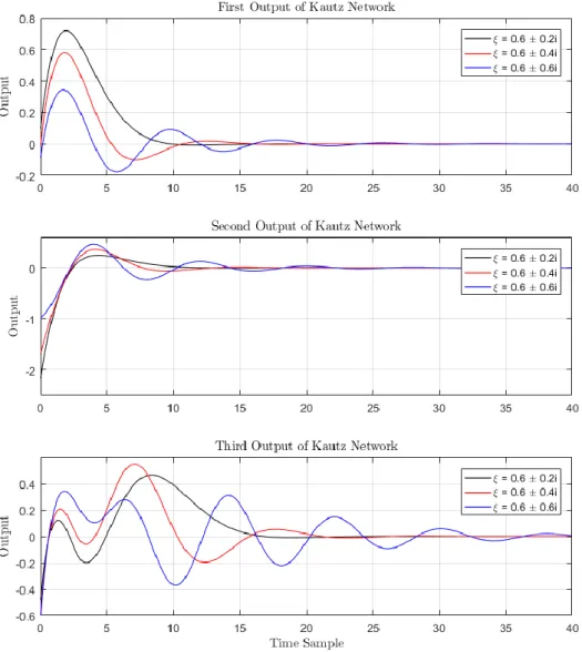
It should be mentioned that the absolute value of the Kautz pole |𝜉| adjusts the decaying rate as well as the oscillation of the Kautz functions. As it is illustrated in Figure 2, a pair of poles with a smaller absolute value indicates a faster convergence to zero while as the magnitude of the poles increases to the boundary of the unit disk, the values of 𝑘𝑖 (⋅)
need more steps to converge to zero. The location of the poles also indicates the number of steps that are needed for achieving the orthonormality of the Kautz network in the state space domain.
The author of [5] used Kautz networks in model predictive control for linear time invariant (LTI) systems. The major virtue, reported by the author, is to decrease the number of decision variables and consequently increase the speed of on-line optimization calculations. The main idea in Kautz parametrization is to consider the control signal as an impulse response of a stable system and then reconstruct it with a Kautz network [5]. Because of the parametrization by a Kautz network, the reconstructed control signal must decay to zero, so we have to convert the control input from 𝑢 to 𝛥 𝑢 by incorporating an integrator into the system (1) and form the augmented system:
[
𝑥(𝑘 + 1)
𝑢(𝑘)
] = [
𝐴(𝑘) 𝐵(𝑘)
0
𝐼
𝑚×𝑚
] [
𝑥(𝑘)
𝑢(𝑘 − 1)
] + [
𝐵(𝑘)
𝐼
𝑚×𝑚] Δ𝑢(𝑘),
(12)
For simplicity, we use the notation
𝑧(𝑘 + 1) = 𝐴
𝑧(𝑘)𝑧(𝑘) + 𝐵
𝑧(𝑘)Δ𝑢(𝑘),
(13)
where 𝑧(𝑘 + 1)𝑇 = [ 𝑥(𝑘 + 1)𝑇 𝑢(𝑘)𝑇] and 𝐴𝑧 (𝑘),𝐵𝑧 (𝑘) are the corresponding matrices to those given in (12).
We will use this model instead of (1) to build the prediction vector (4) and to formulate the optimization problem (5)-(7).
The augmentation (12) makes the system inputs suitable for Kautz network. By this means, the total number of decision variables reduces from 𝑚𝑁𝑝 to ∑𝑚𝑗=1𝑁𝑗 (where 𝑁𝑗 is the degree of the Kautz network used to capture the control signal of channel 𝑗, 𝑗 = 1,…, 𝑚. For every single input 𝛥𝑢(𝑗), 𝑗 = 1,…,𝑚. of (13) we can write:
Δ𝑢
(𝑗)(𝑘) = ∑ 𝑙
𝑞 (𝑗)(𝑘)𝜂
𝑞(𝑗) 𝑁𝑗
𝑞=1
Figure 2. Output of Kautz network in time domain for different pairs of poles
By substituting (14) in (13), we can establish an optimization problem similar to (5)—(7) which is given by
𝐽(𝑥
0) = min
𝑈
𝑋
𝑇
𝑄̅𝑋 + 𝜂
𝑇𝛤
𝑇𝑅̅𝛤𝜂
Subject to 𝑋 = 𝑆
𝑋𝑥
0+ 𝑆
𝑈Γ𝜂
𝐺𝜂 ≤ 𝑔
(15)
Where 𝑋, 𝑄, 𝑅 are defined in (7) and 𝐺, 𝑔 are the corresponding time-varying constraint matrix and constraint vector of the optimization problem. For a system with 𝑚 inputs, the vector 𝜂 and the matrix 𝛤 are defined as
𝜂
𝑇= [𝜂
(1)𝑇𝜂
(2)𝑇⋯ 𝜂
(𝑚)𝑇],
Γ
𝑇= [𝐿(0)
𝑇𝐿(1)
𝑇⋯ 𝐿(𝑁
𝑝
− 1)
𝑇].
𝐿(𝑘) =
[
𝐿
(1)(𝑘)
0
⋯
0
0
𝐿
(2)(𝑘) ⋯
0
⋮
0
⋱
⋮
0
⋯
⋯ 𝐿
(𝑚)(𝑘)]
.
(16)
In (16), 𝐿(𝑝)(𝑘) is the 𝑘′th output of the Kautz network for the 𝑝′th input (𝑝 = 1,…,𝑚) and is given by the left hand side of (11). Solving the optimization problem (15), the unconstrained optimal decision variables 𝜂0 and their
corresponding 𝛥𝑈0 are given by:
𝜂
0= −(Γ
𝑇𝑆
𝑈𝑇
𝑄̅𝑆
𝑈Γ + Γ
𝑇𝑅̅Γ)
−1Γ
𝑇𝑆
𝑈𝑇𝑄̅ 𝑆
𝑋𝑥
0(17)
To solve the constrained solution of (15), we can use conventional quadratic programming packages.
4-
Stability of the Kautz Method in MPC-LTV
In order to show the stability of the Kautz method in MPC for LTV systems we must show that the solution of (15) equals to the solution of (5) under same conditions. In other words, the Kautz network must be able to capture the optimal solution of (6) precisely. Therefore, we have to study under which conditions the Kautz network is able to capture the required optimal input signals. An infinite series of Kautz functions defines a complete set on the z-domain, and any stable transfer function 𝐺(𝑧), can be expressed by the Kautz functions as [18]:
𝐺(𝑧) = ∑ 𝑐
𝑞Ω
𝑞(𝑧)
∞𝑞=1
,
(19.a)
where the 𝑐𝑞's are called the Kautz coefficients. The corresponding representation of (19.a) in the time domain is
𝑔(𝑘) = ∑ 𝑐𝑞𝑙𝑞(𝑘) ∞
𝑞=1
. (19.b)
It is shown in [19] that the necessary and sufficient condition for the completeness of the set Ω𝑞(𝑘) in (10), (19.a) on
𝑙2[0,∞) is
∑(1 − |𝜉|) = ∞
∞
𝑘=0
(20)
Equation (20) means that a finite-energy signal can be approximated with any degree of accuracy by a linear combination of a finite number of Kautz functions. Worded in another way, Equation (20) means that for linear-stable systems, the coefficients of the high order Kautz networks tend to zero, and the system can then be represented by a finite set of Kautz functions. Therefore, in (14), for each 𝑗 there exists a finite 𝑁𝑗 that synthesises the corresponding control signal precisely.
Orthonormality of the Kautz network in the time domain has been proven in [18], and can be expressed as
∑ 𝑙
𝑞(𝑘)𝑙
𝑝(𝑘) = 𝛿(𝑞 − 𝑝)
∞𝑘=0
, 𝑞,𝑝 = 1, ⋯ ,𝑁
(21)
Where 𝛿(⋅) is the Dirac delta-function. In Kautz-based MPC, a truncated version of (21) is employed by replacing
∞ with the prediction horizon 𝑁𝑝. The necessary prediction horizon to achieve orthonormality of a Kautz network is
dependent on its poles, 𝜉,𝜉∗, as well as the network dimension 𝑁 [5]. As the poles 𝜉,𝜉∗ approach the unit circle, a larger prediction horizon 𝑁𝑝 is required to maintain the orthonormality. In a similar manner for larger 𝑁 we need larger 𝑁𝑝 to
preserve this characteristic [5].
The authors of [12] used the optimal cost function of (5) as a Lyapunov function and terminal equality constraint
𝑥(𝑁𝑝) = 0 to provide the general conditions under which stability of model predictive control of a constrained
time-varying nonlinear discrete-time system is guaranteed. Under the assumptions of uniform controllability and uniform observability, it is shown there that the value of the optimal cost function of (5) approaches the value of the infinite horizon problem as the prediction horizon 𝑁𝑝 approaches infinity. We adopt the same assumptions and follow the results
of [5] to establish stability of Kautz parametrization of LTV-MPC. For the sake of simplicity, the stability is established for the case of single-input systems. The extension to multi-input systems is straightforward.
Assumption 1. The final state of the receding horizon optimization problem (15) is constrained to be zero,
𝑥(𝑘 + 𝑁𝑝) = 0, where the terminal state 𝑥(𝑘 + 𝑁𝑝) is obtained from applying the control sequence 𝑢(𝑘 + 𝑚) =
𝐿(𝑚)𝑇𝜂 , 𝑚 = 0, 1, 2, . …, 𝑁𝑝, on system (1). We also assume that 𝑁𝑝 is large enough so that 𝑢(𝑘 + 𝑁𝑝 − 1) = 0.
Assumption 2. For each sampling instant, 𝑘, there exists a solution such that the cost function 𝐽 in (15) is minimized and is equal to the minimized value of 𝐽 in (6).
𝑉(𝑥(𝑘),𝑘) = ∑ 𝑥
0(𝑘 + 𝑚|𝑘)
𝑇𝑄𝑥
0
(𝑘 + 𝑚|𝑘)
𝑁𝑝𝑚=1
+ ∑ Δ𝑢
0(𝑘 + 𝑚|𝑘)
𝑇𝑅Δu
0
(𝑘 + 𝑚|𝑘)
𝑁𝑝−1𝑚=1
(22)
Where 𝑥𝑜(𝑘 + 𝑚|𝑘) = 𝛷(𝑘 + 𝑚,𝑚 − 1)𝑥0+ ∑𝑘+𝑚𝜏=𝑘 𝛷(𝑘 + 𝑚,τ+ 𝑚) 𝐵𝐿(𝑚)𝑇𝜂0, is the optimizer vector of (15)
subject to the constrains. Because 𝑉(𝑥(𝑘),𝑘) is a quadratic function and it is positive definite, it follows that it tends to infinity as 𝑥(𝑘) tends to infinity. In addition, uniform controllability of (1) ensures us that all the elements of system matrix and input matrix remain bounded over the prediction horizon, so the Lyapunov function (22) is bounded from above over time. The same argument can be made for the Lyapunov function at time 𝑘 + 1, that is 𝑉(𝑥(𝑘 + 1),𝑘 + 1). In order to show the monotonic decreasing of the Lyapunov function we can write
𝑉(𝑥(𝑘 + 1)
,
𝑘 + 1) − 𝑉(𝑥(𝑘)
,
𝑘) = −𝑥
0(𝑘)
𝑇𝑄𝑥
0
(𝑘) − 𝜂
0𝑇𝐿(0)
𝑇𝑅𝐿(0)𝜂
0.
(23)
Equation (23) is due to the fact that the principle of optimality (Assumption 2) provides us with the 𝑥𝑜(𝑘 + 𝑚|𝑘) =
𝑥𝑜(𝑘 + 𝑚 + 1|𝑘 + 1) , 𝑢𝑜(𝑘 + 𝑚|𝑘) = 𝑢0(𝑘 + 𝑚 + 1|𝑘 + 1), so all middle terms of 𝑉(𝑥(𝑘 + 1),𝑘 + 1) and
𝑉(𝑥(𝑘),𝑘) cancel each other. For the final terms of 𝑉(𝑥(𝑘 + 1),𝑘 + 1) , 𝑉(𝑥(𝑘),𝑘) we use Assumption 1, hence the asymptotic stability is established.
In the proof of the theorem, we assumed that the Kautz network achieves at each time step the same optimal cost as the conventional MPC method. However, as we will illustrate in the example we are able to achieve stability without achieving optimality. Thus, from a practical point of view, we find that this assumption is usually unnecessary for stability and it could be relaxed. A second line of work is to relax the optimality assumption, and use suboptimal methods to establish stability for the case of LTV systems.
5-
Simulation Example
The example presented here illustrate the effectiveness of Kautz networks in model predictive control of linear time-varying systems. The example considers a single input system and compares the solution of Kautz method (Equation (15)) with the solution of traditional MPC, Equation (6).
Consider the linear system with a time-varying unstable pole that is given by
𝑥(𝑘 + 1) = [
1.05 + 0.2 cos(0.4 𝑘)
0
0.9 + 0.3 sin(0.3𝑘)
2
] 𝑥(𝑘) + [ 0
0.08
] 𝑢(𝑘)
,
(24)
The weighting matrices for this system are taken 𝑄 = 𝑃 = 13𝐼2×2, 𝑅 = 0.1. The prediction horizon is 𝑁𝑝= 16, and
the constraint set for the control and states are |𝑢| ≤ 30, |𝛥𝑢| ≤ 15, ‖𝑥‖∞≤ 8.
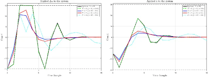
We compare the effect of network dimension and pole value on the behavior of the solution in Figure 3 to Figure 5. In these figures the black-solid line shows the global optimal solution of Equation (6). This solution is achieved with
𝑁 = 10 and an arbitrary value of pole, |𝜉. 𝜉∗| < 1 , in Equation (15). The near optimum solution is drawn in the figures with the green-dashed line that is achieved with 𝑁 = 8; 𝜉 = 0.5 + 𝑗0.15. These two lines captured the optimum solution of system (24) perfectly. However, they do not have a satisfactory dimension network as 𝑁 is too high. The simulation shows that for small vales of 𝑁 the Kautz network is still able to achieve stability. Blue, red and cyan lines are obtained for 𝑁 = 2 that is the smallest possible value (the dimension of the network in Kautz parametrization must be even). The difference between these lines is due to the different selection of pole value. The blue and red lines converge to the origin, though in a different manner compared to the optimal solution. However, the cyan-dotted line is trapped in an oscillation which shows instability. These results illustrate that the effect of network dimension is similar to the effect of control horizon, a larger 𝑁 tends to a closer behavior to the optimum solution. Additionally, the value of
𝜉 is not very influential for large 𝑁 (as we see for 𝑁 = 10). The difference between red, blue and cyan lines indicates that as 𝑁 decreases, the value of 𝜉 becomes important in the terms of stability and optimality.
Figure 3. Applied input for different Kautz Characteristics
been addressed in this paper. It was demonstrated that by means of a Kautz parametrization we can express the future control signals of a time-varying system by a smaller number of decision variables compared to the traditional method. Consequently, the required computation times for solving the optimization problem are decreased as the total number of decision variables decreases, and this constitutes the main advantage of the Kautz parametrization. The stability of Kautz parametrization for MPC of linear time-varying systems was established by means of optimality arguments. In the simulation example, it was verified that even with very small values of N, the Kautz parametrization method preserves stability, which will prompt us to explore the use of suboptimal methods to establish the stability of the scheme. Also, the effects of active constraints, pole location and network degree on the performance of the Kautz-based MPC method were studied through the simulations.
7-
References
[1] A. Bemporad, M. Morari, V. Dua, and E. N. Pistikopoulos, “The explicit linear quadratic regulator for constrained systems,” Automatica, vol. 38, no. 1, pp. 3 – 20, 2002.
[2] M. M. Seron, J. A. De Doná, and G. C. Goodwin, “Global analytical model predictive control with input constraints,” in Proceedings of the 39th IEEE Conference on Decision and Control, vol. 1, 2000, pp. 154–159 vol.1.
[3] L. Wang, “Continuous time model predictive control design using orthonormal functions,” International Journal of Control, vol. 74, no. 16, pp. 1588–1600, 2001.
[4] L. Wang, “Discrete model predictive controller design using Laguerre functions,” Journal of Process Control, vol. 14, no. 2, pp. 131 – 142, 2004.
[5] Wang, Liuping. Model predictive control system design and implementation using MATLAB®. Springer Science & Business
Media, 2009.
[6] J. Rossiter, L. Wang, and G. Valencia-Palomo, “Efficient algorithms for trading off feasibility and performance in predictive control,” International Journal of Control, vol. 83, no. 4, pp. 789–797, 2010.
[7] G. Valencia-Palomo and J. A. Rossiter, “Novel programmable logic controller implementation of a predictive controller based on Laguerre functions and multi-parametric solutions,” IET Control Theory Applications, vol. 6, no. 8, pp. 1003–1014, May 2012. [8] B. Khan and J. A. Rossiter, “Robust MPC algorithms using alternative parameterizations,” in International Conference on Control (UKACC). IEEE, 2012, pp. 882–887.
[9] W. Kwon and A. Pearson, “A modified quadratic cost problem and feedback stabilization of a linear system,” IEEE Transactions on Automatic Control, vol. 22, no. 5, pp. 838–842, Oct 1977.
[10] “On feedback stabilization of time-varying discrete linear systems,” IEEE Transactions on Automatic Control, vol. 23, no. 3, pp. 479–481, Jun 1978
[11] W. H. Kwon, A. M. Bruckstein, and T. Kailath, “Stabilizing state-feedback design via the moving horizon method,” International Journal of Control, vol. 37, no. 3, pp. 631–643, 1983.
[12] S. S. Keerthi and E. G. Gilbert, “Optimal infinite-horizon feedback laws for a general class of constrained discrete-time systems: Stability and moving-horizon approximations,” Journal of Optimization Theory and Applications, vol. 57, no. 2, pp. 265–293, 1988. [13] D. Q. Mayne and H. Michalska, “Receding horizon control of nonlinear systems,” IEEE Transactions on Automatic Control, vol. 35, no. 7, pp. 814–824, Jul 1990.
[14] G. D. Nicolao, L. Magni, and R. Scattolini, “Stabilizing receding horizon control of nonlinear time-varying systems,” IEEE Transactions on Automatic Control, vol. 43, no. 7, pp. 1030–1036, Jul 1998.
[15] P. Falcone, F. Borrelli, J. Asgari, H. E. Tseng and D. Hrovat, "Predictive Active Steering Control for Autonomous Vehicle Systems," in IEEE Transactions on Control Systems Technology, vol. 15, no. 3, pp. 566-580, May 2007.
[16] E. W. Kamen, The Control Handbook: Control System Advanced Methods, 2nd ed. CRC Press, 2010, Fundamentals of Linear Time-Varying Systems.
[17] Wahlberg, B, “System identification using Kautz models,” IEEE Transactions on Automatic Control, 39(6), 1276-1282, Jun 1994.
[18] Oliveira, G. H., da Rosa, A., Campello, R. J., Machado, J. B., & Amaral, W. C. “An introduction to models based on Laguerre, Kautz and other related orthonormal functions– part i: linear and uncertain models,” International Journal of Modelling, Identification and Control, 14(1-2), 121–132, 2011.