Learning Rare Patterns with Multilevel Models.

(1)

ABSTRACT

RAVINDRAN, SRINATH. Learning Rare Patterns with Multilevel Models. (Under the direction of Dennis Bahler.)

In applications of machine learning as diverse as computer vision, information re-trieval, text classification, chemoinformatics, and bioinformatics, a variety of common issues have been identified involving frequency of occurrence, variation and similarities of examples, and lack of examples. These issues continue to be important hurdles in ma-chine intelligence and this work focuses on developing robust mama-chine learning models that address the same. In particular, the approaches we discuss in this work fall under the general framework of Multilevel Models. Recent research has shown that multilevel and hierarchical models are well suited for finding solutions to learning in the presence of complex data.

We are interested in utilizing the power of multilevel models to solve the problem of learning in the presence of a small number of examples. Unsupervised learning algorithms such as k-means clustering and Dirichlet process mixture models can be used to identify similarity between the data points and form meaningful clusters from them. Such algo-rithms can also be used to place the rare example in appropriate groups, and such an assignment can be used further to learn the concept.

(2)

rareness.

(3)

(4)

Learning Rare Patterns with Multilevel Models

by

Srinath Ravindran

A dissertation submitted to the Graduate Faculty of North Carolina State University

in partial fulfillment of the requirements for the Degree of

Doctor of Philosophy

Computer Science

Raleigh, North Carolina

2017

APPROVED BY:

Jon Doyle James Lester II

Munindar Singh Dennis Bahler

(5)

DEDICATION

(6)

BIOGRAPHY

Srinath Ravindran was born in Coimbatore, a city in the state of Tamil Nadu, India. He grew up in Chennai, the best city in the world, and also the state capital of Tamil Nadu. He finished high school at Bala Vidya Mandir, Chennai and received his Bachelor of Engineering degree in Computer Science and Engineering from Anna University, Chennai in 2007. He received a Master of Science degree in Computer Science from North Carolina State University (NCSU), Raleigh, in 2009.

(7)

ACKNOWLEDGEMENTS

I take this opportunity to express my gratitude to the people who directly or indirectly contributed to the completion of this thesis.

First, I would like to thank my advisor, Dr. Dennis Bahler for his guidance, support, and patience. He encouraged me to work on interesting projects in addition to my disser-tation, pursue internships, and teach courses. Next, I would like to thank my committee members, Dr. Jon Doyle, Dr. James Lester, and Dr. Munindar Singh. I am grateful that they all agreed to be part of my doctoral committee.

Dr. Thuente, Dr. Reeves, and Dr. Rouskas served as the Directors of Graduate pro-gram during my years in grad school, and I thank them for their guidance, and encour-agement. I would be remiss if I do not thank Dr. Christopher Healey and Dr. Robert St. Amant. I have worked with them on several occasions, and have learned a lot through the interactions.

I have spent a lot of time at the Knowledge Discovery Lab to an extent that it was my second home. I’ll always remember the late nights, open houses, presentations, broken refrigerators, video games, cricket world cup, and more. My stay in the lab was made memorable by a lot of people: Thomas, Lloyd, Marivic, Kyung Wha Hong, Lihua Hao, Joe Hsiao, Andrew Wicker, Shea McIntee, Karthik, Nazli, Prairie Rose, and Adam Marrs. I extend a special thanks to my grad school friends: Reuben, Arun Prakash, Alex Jamestin, Supritam Sen, Arpan, Trisha, Sina Bahram, Hilay, Kalpesh, Lifford, Vineha, and Pradeep Murukanaiah.

(8)

LIST OF TABLES

Table 4.1 Comparison of RMSE values for Toxicity Data . . . 70 Table 4.2 Description of Datasets . . . 71 Table 4.3 RMSE on UCI and Delve regression datasets: Comparing the

per-formance of our approach with other approaches to regression . . . 74 Table 4.4 Normalized Error: error values normalized with respect to the

per-formance of SBMM . . . 74 Table 4.5 Number of rare examples correctly predicted within 1% error margin 75

Table 5.1 Description of Datasets . . . 88 Table 5.2 Precision and Recall on UCI and Delve Classification datasets:

Com-paring the performance of our approach with other common ap-proaches . . . 91 Table 5.3 Learn a rare example and testing on more examples from the “rare

(11)

LIST OF FIGURES

Figure 2.1 Example xi, belongs to class C. δi is the deviation and FC is the

frequency of class C with respect to the dataset. δi is measured

from the centroid ofC. FC = 9/|D| . . . 20

Figure 2.2 Value of R: δi -X axis, (1−FC) - Y axis, R - Z axis. m = n = 3

and m=n= 7 . . . 23 Figure 2.3 Relationship betweenError(M SE),V ariance and Bias2 . . . 25 Figure 2.4 Long Tail . . . 28

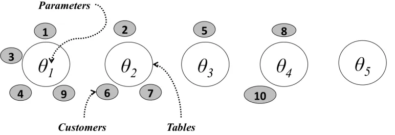
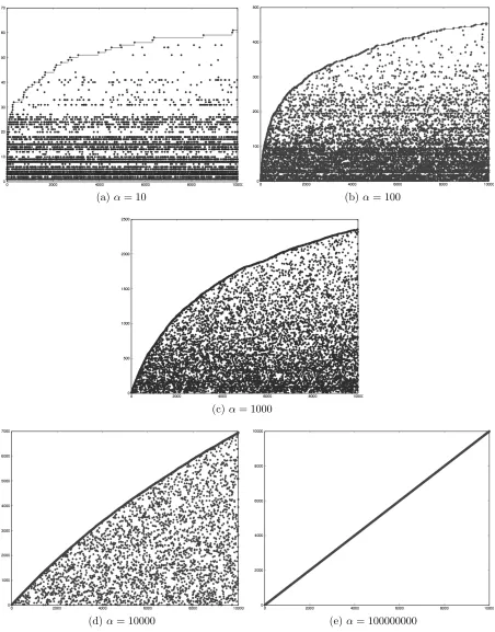
Figure 3.1 Chinese Restaurant Process. Customers are distributed in tables according to the probabilities in Equations 3.11 and 3.11 . . . 51 Figure 3.2 Variation of number of elements in each cluster for different values

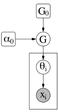
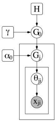
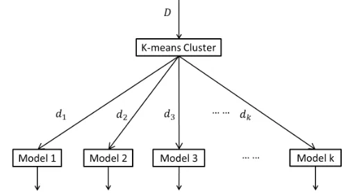
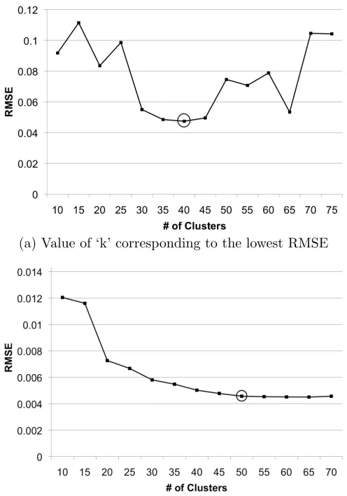
of α. For smaller values of α, crowded tables attract more cus-tomers, whereas larger valuers of α yield a more uniform distribu-tion of the customers across the tables. . . 53 Figure 3.3 Plate Model for the Dirichlet Process Mixture Model (DPMM) . . 54 Figure 3.4 Hierarchical Dirichlet Processes Mixture Model (HDPMM) . . . . 58 Figure 4.1 Similarity Based Multilevel Model (SBMM) . . . 61 Figure 4.2 Two types of curves for RMSE vs Number of clusters . . . 63 Figure 4.3 Time taken to train the model with increase in number of clusters. 65 Figure 4.4 Data Clusters . . . 67

(12)

Chapter 1 Introduction

There are a variety of machine learning approaches that work well for problems involving independently and identically distributed (IID) data, and cases with enough examples to represent the variations in data. However, in many practical applications including computer vision, text classification, bioinformatics, and others, we may not have sufficient examples, the data may not be drawn from identical distributions, or there could be complex relations among individual data points.

These problems that make the learning task difficult and often error prone typically fall under the following categories:

1. Within-class Variation and Inter-class Similarity: examples within one category or class have different properties, whereas examples from different categories or classes may have similar properties.

2. Lack of Good Quality Examples and Rare Examples: examples that either belong to an unknown class or are assigned an imprecise class label.

(13)

be present in either training or test data.

Over the past few years, a variety of approaches have been developed to address each of the issues mentioned above. Existing approaches to prediction most often do not consider these problems together, instead treating these as separate problems. However, there are many applications having some combination of these problems.

An example application is chemical toxicity prediction. Chemicals belong to various congeneric classes such as acids, alcohols and amines. Often the chemicals in one class exhibit properties similar to chemicals in another congeneric class while being different from chemicals in the same class. The former phenomenon is an example of within-class variationand the latterinter-class similarity. Moreover, the occurrence of some chemicals may be rare or unseen. That is, the chemical may be the only representative of its class in the training data, or a chemical that is not be present training set could be presented at a later stage (test set) for a prediction task. Finally, the labels assigned to each of the chemicals are determined experimentally and this task is costly and, as often in other applications, error prone.

(14)

1.1 Terms and Definitions

We will use several key words or phrases across all the chapters in this document; we present them in this section. We have tried to make the usage of terms consistent across chapters, while not departing from some of the conventions used in the literature.

In machine learning problems, we are presented with a data set, we would like to learn from. For instance, in order to learn to recognize hand-written digits, the dataset will contain several images of digits 0-9, each written by a person with pen and paper. Some examples of such a dataset include MNIST [42] and the Hand-written digit recognition datasets [5]. Every image of each digit is called a data point, instance, an observation, or an example. In our work we will use the term example to collectively represent these terms. Generally, each dataset D has a finite set of such examples, and the number of examples is denoted byN. The number of examples in a set of examples is also denoted by |D|. A subset of examples that exhibit common or similar features are referred to as a pattern.

For the problem of recognizing hand-written digits, the learning algorithm must learn the digit based on the examples in the dataset. Examples of each digit share some visual similarities with each other, and at the same time are visually different from the other digits. The visual similarities and differences are represented by features or attributes. In case of the images representing digits, the line segments that make up the outline of the digits are one of the features. If we consider the set of examples representing the number 4, people have different ways of writing the number, and each of those variations constitute a pattern.

(15)

labels are referred to as Class Labels, and the images of a certain digit, say 5, are said to belong to class 5. The literature uses the terms classes and categories interchangeably, and we will use the term classthroughout the document.

More formally, let us assume that we are given training data _T consisting of N ex-amples, where each example xi has a label yi. The set of examples is represented as

{(x1, y1),(x2, y2), . . . ,(xn, yn)}. The learning task is then to produce a classifier h:X →Y

which maps an object x ∈ X to its class label y ∈ Y. Each example, xi is often

repre-sented by a_D-dimensional feature vectorx= (xi1, . . . , xiD)∈RD. Each dimension in the feature space represents a feature or attribute, and xi is a point in the feature space.

It is important to note that the dataset represents only a sample of examples, and not the entire population. The dataset, therefore, will not reflect the population nor mimic the distribution of examples in the population. For instance, while the digit zero (0) might occur more frequently than other digits in real life, the data set could consist of the same number of examples for each digit.

1.2 Our Work

This research aims to study the following:

1. Learning in the presence of a small number of examples

2. Feature representation techniques to aid learning in complex scenarios

(16)

of the nature of the problem or the cost involved in gathering them. These examples occurring with low frequency could be

1. A new sub-class of a known class

2. The first occurrence of a newly discovered class

3. The only known examples of some class

Each of these problems is commonly studied under topics such as rare examples [62], class imbalance [35], transfer learning [50], and dataset shift [56]. We discuss the relationship among these problem in Section 2.2. We also briefly discuss the effects of rare data and small number of examples in the context of transfer learning and hierarchical models [61]. We have identified ways in which rare data can affect performance in transfer learning and hierarchical models.

These problems are not relevant only in traditional machine learning problems but also within the current trend of “Big-Data”. While big-data problems in general deal with handling large amounts of data, the aforementioned problems are still present.

In the context of big-data, one might also have come across the phrase “needle in the haystack” used as an umbrella term to describe all these problems. We feel that the term does not do justice towards helping the community understand the problems. This is just the tip of the iceberg and there are a variety of such misused and misunderstood terms that affect further research. One of the contributions of this work is toward resolving these issues. We continue this discussion in Chapter 2.

(17)

Simi-larity Based Multilevel Model (SBMM) for Regression in Chapter 4, and Classification Models for Learning Rare Data in Chapter 5.

SBMM is a multilevel regression model that uses the similarity among data points to effectively predict the target values for a new example. Data points within a cluster or within the same neighborhood are considered similar to each other. The approach is based on the assumption that any datapoint has some degree of similarity to some subset of previously known data points.

The Similarity Based Classification Model in Chapter 5, like the SBMM, uses the similarity among the data points to classify them. When presented with a rare example, the model either assigns a new class label, or an existing class label, based on how similar the example is from the previously learned examples.

Both the models work well when there is sufficient background knowledge. Once a model is pre-trained with labeled examples, it is presented with a new example to learn. As we will show in the respective chapters, the models are not only able to learn the new example, but also predict future examples with high accuracy.

(18)

Chapter 2 Learning with a Small Number of

Examples

2.1 Introduction

Traditional machine learning assumes the availability of a large number of examples for every possible class involved in the learning problem. The crux of our work lies in improving predictive performance when the data contains a small number of examples. Learning in such settings has attracted attention in recent times for a variety of reasons.

1. Cognitive: Humans have the ability to learn or generalize concepts with as few as one example, given sufficient background knowledge.

2. Practical: Gathering examples involves scientific experimentation, exploration of the environment, etc.

(19)

While this list is not comprehensive, it provides good motivation to study this topic. Lack of data can be perceived in various forms including rareness, imbalance, missing data and sparsity, and each of these affect learning in different ways. This problem is still relevant in the era of big data.

In this chapter, we discuss different types of learning scenarios involving a small number of examples. We provide insights from existing literature and present our findings as well. In the process, we resolve conflicting terminologies. For example, there is a significant misunderstanding of some concepts, including the use of the term “rare”. Sometimes rare data is used to mean class imbalance, while sometimes it is used to refer to examples that occur infrequently.

We also discuss the relationship among concepts in machine learning such as data shift, imbalance, rareness and missing data.

2.2 Small Number of Examples

Learning in the presence of a small number of examples is an important problem and there are many issues that require attention. In many learning scenarios, obtaining sufficient examples is hard either because of the nature of the problem or the cost involved in gathering them. These examples occurring with low frequency could be

1. A new sub-class of a known class

2. The first occurrence of a newly discovered class

3. The only known example(s) of some class

(20)

1. Number of Examples: Based on the number or proportion of examples in the training set.

In some problems, the number or proportion of examples in the training set can be different for different classes. One very common example is that ofClass Imbalance, where given two classes C1 and C2, the number of examples of C1, represented as

|C1|, can be significantly more than the number of examples of classC2, represented

as |C2|. Such datasets are also called skewed datasets. Class imbalance can be

generalized to multi-class classification problems.

Apart from class imbalance, lack of examples in the training set presents itself in other forms such as rare examples and missing information.

An extreme problem in this category is One-shot Learning, where we learn a new class using only one example, given sufficient background knowledge.

2. Training Phase vs Test Phase:Based on the existence of examples in the train-ing set or test/ classification set.

A lack of examples or presence of a rare example can exist either during training phase or the test phase. Ideally, one would expect statistical models to be capable of learning concepts even from under-represented classes and also to predict unseen examples with great accuracy when the model is used. In reality, however, this is harder to achieve.

(21)

or there may not be enough preexisting knowledge about the class of the example being considered.

Achieving a good balance between bias and variance at training time is often the primary weapon of choice when dealing with lack of examples. There is no one definite solution as this problem is domain and problem dependent.

3. Feature Space: Based on differences in the features and values of the attributes among examples.

Datasets with complete data are easier to learn from compared to complex or incomplete datasets. Often, the complexity in the dataset is due to the feature set. The choice of features, lack of values for the features and variance in the values of the features are all typical reasons for the complexity.

In several learning scenarios, the choice of features is a major problem. Ease of collecting data, cost effectiveness of some features, and lack of sufficient domain knowledge can lead to poor choice of a feature set. Such a choice can worsen the learning problem in an already skewed dataset.

2.2.1 Class Imbalance

In many real-world applications the problem of learning from imbalanced data has at-tracted growing attention from both academia and industry. Learning with imbalanced data is concerned with learning algorithms that work in the presence of underrepresented data and class distribution skews. Any data set that exhibits an unequal distribution of examples between its classes can be considered imbalanced.

(22)

1. Relative or between-class imbalance

2. Imbalance due to rare examples and within-class imbalance

3. A combination of imbalanced data and small sample size

The most common type of imbalance is Between-Class Imbalance. An unbalanced dataset contains significantly more examples in one class than in the other classes. For example, in a binary classification problem with two classes “A” and “B”, class “A” could outnumber class “B” by a large factor and orders such as 10000:1 are not uncommon. The same can be extended to multi-class classification problems. The under-represented class is referred to as the Minority Class.

Class imbalance affects the performance of the classifier. In many cases, the classifier is unable to learn the minority class effectively due to the lack of examples. Minority classes occur in a variety of application domains, including identifying fraudulent credit card transactions, text categorization, detecting certain objects from images and predicting cancer, to name a few. In each of these applications, the minority class is the one of greater importance, and the accuracy of classification is, in many cases, a matter of life-or-death. A naive classifier would learn the majority class well, but is unable to learn the minority class extensively due to a lack of examples. A new example from the minority class is more likely to be misclassified with such a naive classifier.

Much of the published work in machine learning addresses relative or between-class imbalance. Techniques have been developed for learning in the presence of imbalanced data [19, 35].

Class imbalance can be a result of several factors and we list a few here.

(23)

In several domains, examples of some classes are naturally fewer in number com-pared to other classes within the same problem domain. In such cases, identifying more examples of the minority class may be close to impossible.

2. Exploration of the Problem Space

In some scenarios such as processing streaming data, the distribution of incoming data could be such that examples of one of the classes could arrive later in the stream. As a result, early in the process, or at a given time interval, such a class might appear to be a minority. However, over time, it is possible for the dataset to be better balanced.

3. Cost of Exploration

The cost of collecting data is usually high for most domains. For scientific domains, the data collection often involves long hours in a laboratory setting or on-field sensing. The cost is even higher when labeled data is required.

4. Choice of Features

While the skewed class distribution causes the imbalance, in some scenarios, the choice of features or the set of recorded attributes may be bad enough to make learning harder than it is if the data processing was performed with different choice of features.

Class Imbalance Can be a Good Thing

In some real life classification tasks, having a skewed dataset, where|C2|>>|C1|, can be

(24)

using multiple binary classifiers. We might use a classifier for music, movie, travel, video games etc. Suppose we would like to build a classifier to identify if the search query is about a video game. An easy approach is to collect a set of search queries that led the user to click a video game webpage, the set of positive examples C1, and search queries

that did not lead to a video game webpage, the set of negative examples C2. Since video

game titles often have similar name or shared keywords, the n-grams formed by the words in the movie title can be used as the feature set.

In this case, it is desirable to have more negative examples than positive examples, or

|C2| >> |C1|. That way, the classifier can precisely identify video game titles and have

lower risk of misclassification.

Apart from showing that class imbalance is not necessarily evil, the example also highlights another important point. Traditionally, research on class imbalance has been concerned with the frequency of occurrence of the examples. However, as demonstrated by the example above, given a rich enough feature space and the requirement of the clas-sifier to avoid misclassification, having a skewed dataset may not be as bad as generally believed.

Further, in some problems, the learning becomes easier when the dimensionality “d” is large. Several studies have studied binary classification problems that are “easier” when d is large [39, 52]. Dicker and Foster [23] show that the prediction is easier when the dimension of xi is large since that provides more context in regression problems.

2.2.2 One-Shot Learning

(25)

scenario wherein a model is able to learn or generalize a concept or a category Ci using

as few as one example from Ci, given some background knowledge. Existing approaches

initially build a model using a large initial dataset, which acts as prior knowledge of the domain. When an example from an unseen class is presented, the model learns the class using the information supplied by the existing model and based on the new example’s similarity to previously learned examples.

An older approach, Explanation Based Learning (EBL) [22], also learns from one example and in a sense is very similar to one-shot learning as it is known today. EBL requires a domain theory, which needs to be consistent and complete, a training example, a goal concept and an operationality criteria. EBL generalizes the training example such that the generalization is consistent with the goal concept and meets the operationality criteria. Among the various issues with EBL, defining the operationality criteria is not easy.

2.2.3 Dataset Shift

In real world applications, the conditions in which we use a statistical model differ from the conditions that existed when training the model for several reasons. Dataset shift deals with such differences by relating information in very similar or related environments or tasks to help in the prediction of one task given the data or prior knowledge in the others. As noted in [56], there are several flavors of dataset shift.

1. Simple covariate shift occurs when only the distributions of the covariates change and everything else is the same.

(26)

3. Sample selection bias occurs when the distributions differ as a result of an unknown sample rejection process.

4. Imbalanced data is a form of deliberate dataset shift for computational or modeling convenience.

5. Domain shift involves changes in measurement. Source component shift involves changes in strength of contributing components.

2.2.4 Domain Transfer

Domain Transfer, or transfer learning is motivated by the fact that humans can apply knowledge learned previously to solve new problems that might arise in similar or related tasks, faster or with higher accuracy. In 2005, DARPA [21] defined transfer learning as the ability of a system to recognize and apply knowledge and skills learned in previous tasks to novel tasks. Thus, there are two sets of tasks: a source task, from which the learning system learns and a target task, to which the acquired/learned knowledge is applied. The source and target tasks need not be the same, but are related in some sense. This is in contrast with traditional machine learning approaches which require the source and the target tasks to be the same.

(27)

2.3 Rare examples

Unbalanced data [35, 55, 62] and its effects have been a topic of interest for a long time in supervised learning. Almost any real world application suffers from the effects of unbalanced data. As noted in [35], there are different types of imbalances and three specific types of imbalances are more prominent:

1. Relative or between-class imbalance

2. Imbalance due to rare examples and within-class imbalance

3. A combination of imbalanced data and small sample size

Much of the published work in machine learning addresses relative or between-class imbalance. Techniques have been developed for learning in the presence of imbalanced data [19, 35] where the number of examples in class C1 greatly exceeds the number of

examples in classC2. Further, some multilevel approaches [77] are known to aid prediction

in the presence of data imbalance. Many approaches artificially “balance” the imbalanced datasets by sampling. Some of these approaches either deliberately or unintentionally compromise overall performance to achieve good approximation on rare examples [19, 35, 55].

(28)

Relatively, there is more work on detecting rare events or rare examples, than there is on prediction tasks. Past research has concentrated on detecting rare cases from a set of examples, especially in streaming data [74]. Only a handful of the existing approaches study learning in the presence of rare examples [62]. There are some issues of both theoretical and practical importance that affect progress.

In our investigation, we have found that many of the existing algorithms are unable to provide good approximations for examples that are rare or under-represented in the training set. For example, it is important to predict the toxicity of a chemical that belongs to an unknown chemical class or functional group accurately while preserving, or even the overall accuracy of our model. Further, the presence of within-class variation and inter-class similarity affects the performance of a machine learning model. When compared to traditional techniques, our approach achieves better performance on such data without compromising the overall error rate.

Moreover, there are two more problems with existing definitions of imbalance and rareness. The existing approaches are based on:

• Frequency only: All definitions of imbalance are based on frequency of occurrence

of the examples in the dataset. In a two-class classification problem, given two classesC1andC2, the number of examples ofC1, represented as|C1|, is significantly

more than the number of examples of class C2, represented as |C2|.

However, as discussed earlier in Section 2.2.1, frequency alone cannot be used to define imbalance. In datasets with within-class imbalance, this definition and ap-proaches based on the definition, are more likely to have higher error rates. Classi-fiers must take features into account.

(29)

are considered as a 0-1 thresholds as illustrated in the Equation below.

R=     

0 for C1 < T

1 for C1 >=T

(2.1)

Where, R is the degree of rareness or imbalance,T is the threshold to determine if the dataset is imbalanced. Typical values of T are 1%, 5%,. . . 30%.

In the next section, we provide a quantitative representation of rareness.

2.3.1 Quantifying Rareness

Currently, imbalance and rareness are defined as a function of the data frequency. Data points that occur less frequently are considered rare. Likewise, in a classification problem, the dataset is considered unbalanced if one of the classes has fewer examples compared to the other classes. There is a general belief that an unbalanced dataset is hard to learn from, where the value of learning is measured by a combination of the ability of the learning algorithm to learn efficiently, and to predict new examples with high accuracy.

In practice, however, there are problems where a 75-25 imbalance is easy to learn, while the same imbalance can be hard to learn in other cases. Primary differentiating factors include the choice of features and the quality of the examples. Generally, if the features are descriptive of the dataset, the learning problem is easier, and we can generalize with higher accuracy. In several real life situations, obtaining such features may not be easy for several reasons such as those discussed in Section 2.2.

(30)

out of 100 examples are different from the rest of the examples, they are rare to a high degree. If 50 out of 100 examples in a class are different from other examples in the same class, they are “rare” to a small (but non-zero) extent.

A distance measure such as Euclidian distance can be used to determine how much an example is different from, or deviates from the other examples. The distance of an example xi is either measured from the centroid of set of examples belonging to a class

Ck, or is measured pairwise between allxiand all other examples. The choice of approach

depends on the application. In order to determine rareness, we measure the distance of an example from the centroid.

Defining Rare Examples Based on the our observations, we can define rare examples or patterns as follows:

“An example xi belonging to a class C in the given dataset D is considered rare if

xi deviates more from the centroid than other examples in classC, and the frequency of

class C, FC is small, i.e.,|FC| |D|.”

In order to illustrate this, let us consider the problem of detecting cancer. Let classC represent all known cases of cancer in the dataset. The number of examples of “cancer” is relatively low compared to the number of examples of “not cancer”. Now, ifxi represents

a new form of cancer that was recently detected, then xi will be considered rare.

The definition of rareness can be further generalized to describe rareness in a hierarchy of classes. That is, ifxi is an example of a subclass ofC that occurs with low frequency,

and xi is different from the rest of the examples, then it is considered rare. Let us

(31)

cultural differences, or can be result of personal habit. Let us consider the set of examples of the number 4. There are several variations or patterns of writing 4. For instance, some people leave the top “open” like in the seven segment display, while others use a “closed” top. If the examplexi represents one of these variations 4, then it is different from rest of

the examples of the number 4. xi is considered rare if the variation it represents occurs

with low frequency with respect to the overall frequency of all examples representing the number 4.

Thus the definition covers the different kinds of imbalances: between class and within class imbalances; we described these earlier in Section 2.2.1.

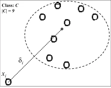
Figure 2.1: Example xi, belongs to class C. δi is the deviation and FC is the frequency

(32)

The degree of deviation between the example xi is denoted by δi ∈R. FC denotes the

frequency of occurrence of the setV, wherexi ∈V. Figure 2.1 illustrates the idea.

The rareness measureRi for an examplexiis then obtained by a combination ofδi and

FC. The user defines rareness based on the application. We use the following rationale to

obtain Ri. We use T to represent the threshold of frequency.

1. FC ≥ T and small values δi: The example in the dataset is related to the rest of

the examples in the class, and the class has sufficient representation.

2. FC < T and small values δi: The examples in the dataset are related but the

evidence of occurrence is low – aninfrequent pattern.

3. FC = 0: The example has not appeared yet in the dataset. δi is undefined in this

case.

4. FC ≥T and large values of δi: In spite of high frequency of occurrence, the example

may not be related to the others in the dataset.

5. FC < T and large values of δi: a rare example.

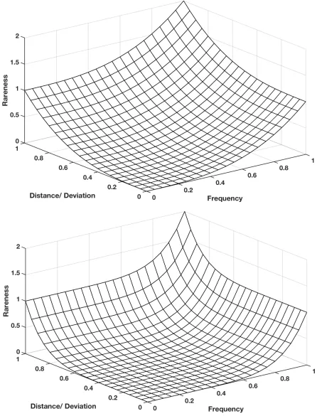
Using the above rationale, we derive the values of R. A simple equation such as the one shown below can help us realize the rationale in a 3-dimensional Euclidean space. We can express rareness of example xi in classC with the following function:

Ri =δim+ (1−FC)n (2.2)

(33)

high relationship (δi). We can determine the amount of rareness by appropriate choice of

values m and n.

The 3-dimensional plot in Figure 2.2 describes the value of R (along the Z axis). In this 3d plot, 0 ≤ δi ≤ 1 and 0 ≤ 1−FC ≤ 1. The same can be generalized to larger

values as well.

The degree of rareness from Equation 2.2 serves two purposes.

• We can identify rare examples from a dataset such as those used in the experiments

from Chapters 4 and 5.

• The degree of rareness can used as a parameter when learning a classification model

in Chapter 5.

2.4 Challenges in Learning with Small Number of

Examples

Learning with a small number of examples is not without challenges. Understanding some of these is key in solving the problem. Over the years, some of these challenges have been better understood, theories have been developed to effectively solve several other, while still others remains an open area for research. In this section, we highlight some of the primary pitfalls and challenges that one needs to remember when learning with a limited number of examples.

2.4.1 Bias-Variance Tradeoff

(34)

Figure 2.2: Value of R: δi -X axis, (1 − FC) - Y axis, R - Z axis. m = n = 3 and

(35)

one of the primary concepts in machine learning. In short, if the hypothesis space is too small and/or simple for the application, in general there will be high bias but low variance. On the other hand, if the hypothesis space is too large and/or complex for the application, in general there will be low bias but high variance.

When presented with a rich dataset containing sufficient examples to represent each concept, the model will be able to learn the concepts well. In such cases, however, we still run into the risk of learning a very complex model, or a model with very high variance. Predictive accuracy is low in such models as well, and the accuracy decreases with increase in model complexity.

In learning problems involving a small dataset, the model will have high bias. Since the data set to learn the concept is limited, the model has limited opportunity to fully capture the various nuances of the concept in its entirety. This in turn affects the predictive accuracy of the model since future examples are not guaranteed to be exact replicas of the data point or points used to learn the concept. Since we are interested in learning rare concepts, handling high bias is important, as is ensuring a balance between bias and variance.

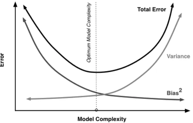
A model that is able to simultaneously minimize bias and variance generally has the highest accuracy. In a learning problem, if t is the unknown correct value, ˆt is the predicted value, andE[ˆt] is mean predicted value over all possible training sets, then

Bias(ˆt) = (E[ˆt]−t) V ariance(ˆt) = E[(ˆt−E[ˆt])2]

(2.3)

Typically, in prediction problems, we minimize the Mean Squared Error, or MSE.

(36)

The above Equation 2.4 can be rewritten as follows:

M SE =E[(ˆt−t)2] =E[(ˆt−E[ˆt] +E[ˆt]−t)2]

=E[(ˆt−E[ˆt])2+ (E[ˆt]−t)2+ 2(E[ˆt]−t)(ˆt−E[ˆt])] =E[(ˆt−E[ˆt])2] +E[(E[ˆt]−t)2] +E[2(E[ˆt]−t)(ˆt−E[ˆt])]

=E[(ˆt−E[ˆt])2] + (E[ˆt]−t)2 =V ariance(ˆt) +Bias(ˆt)2

(2.5)

Note that because (E[ˆt]−t) is a constant and (ˆt−E[ˆt]) = 0, the MSE simplifies to a sum of variance and the square of the bias. Thus, minimizing both bias and variance results in low error, or high accuracy. Figure 2.3 illustrates this relationship.

(37)

When learning from rare concepts, minimizing bias is a challenge. In some cases, as we obtain more examples to represent the rare concept, retraining the model is one way to reduce bias. In Chapters 4 and 5, we will discuss how our models are able to improve predictive accuracy with a simplest possible model, thus achieving a good balance between bias and variance.

2.4.2 Noise vs. Rare Data

In general, noisy examples and rare data points are very similar, and in some cases practically indistinguishable. There are several ways to handle noise in datasets.

• Treat noise as a rare example – we can treat the noisy example as a representative

of an extremely rare class. In many applications, the rare example is contradictory to already known facts. While it is easy to discard the rare example as noise, but in doing so we lose information carried by that example.

• Ignore the noisy example – Probably the simplest thing to do is to ignore noise, and

learn the other concepts in the dataset. While this is a safe option when learning a simple model, we must have a good mechanism to identify or isolate noise from the rest of the data. In some cases, the learning algorithms themselves are robust to noise.

• Correct the noise – Correcting noise requires either reacquiring one or many of the

(38)

2.4.3 Obtaining Sufficient Examples, and Good Quality Class

Labels

A rare example, by definition, occurs less frequently than other examples in the problem space, and is often different from the already known examples. In such cases, an expert’s supervision is required in order to obtain the correct target value. Techniques such as Active Learning and Semi Supervised learning are often employed to obtain the class labels. However, due to the nature of the problem, this challenge remains.

2.5 Related Concepts

There are several concepts related to rare examples, and it is important to understand their similarities and differences with respect to our work. In particular, we would like to highlight three of the most prominent concepts.

2.5.1 Long Tail

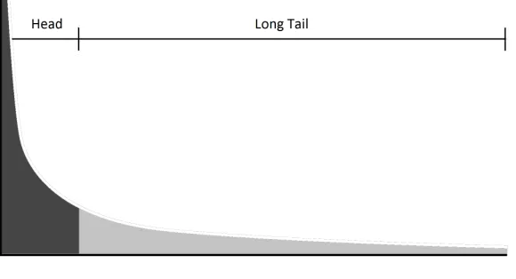
The Long Tail is a well known phenomenon wherein a small number of generic ob-jects/entities/words appear very often and most others appear more rarely. Long tail is a term used in variety of domains ranging from media, online business of search and ad-vertising, economic models and marketing. The “tail” is the part of a distribution having several examples or occurrences with low frequency and the “head” is the part showing occurrences with higher frequency. A typical “long tail” distribution is shown in Figure 2.4.

(39)

Figure 2.4: Long Tail

In search engines, the distribution representing the frequency of searches for keywords or queries is considered long tail. That is, a small number of keywords or queries are searched for with very high frequently in a given time period and a large number of other keywords or queries are searched for with relatively low frequency. The former set of keywords constitutes the head and the latter set of keywords forms the long tail. For instance, during a major sporting event like the super bowl, keywords such as NFL, Super Bowl, NFC, AFC, Super Bowl MVP, Super Bowl Ads etc., would be part of the head. The tail might consist of queries such as “Discovery of the 9th planet”.

Related concepts include the Power law, Zipf’s law [28], and Pareto distribution. Power laws deal with the frequency of distribution of items, and can be observed in a wide range of applications. A power-law probability distribution is a distribution whose density function (or mass function in the discrete case) has the formP(X > x)∼x−α+1_,

where α >1.

(40)

the frequency table for the domain. One application is the study of how terms are dis-tributed across documents. If the most frequent term occurs f1 times, then the second

most frequent term occurs half as many times (f2 =f1/2), the third most frequent term

a third as many occurrences (f3 =f1/3), and so on. In general, fi = f1/i for i=1,2,. . . ,

n. Thus frequency decreases very rapidly with rank. Zipf’s law is a discrete distribution, and can be represented by a Zeta Distribution.

The Pareto distribution is similar to Zipf’s law but is a continuous distribution. Pareto’s law is given in terms of the cumulative distribution function (CDF) and it represents the number of items larger than x is an inverse power of x: P[X > x]∼x−k. The Pareto principle, or the 80-20 principle is a special case of the Pareto distribution.

2.5.2 Cold Start

The cold start problem is common in inference engines and recommendation systems where the system cannot draw meaningful inferences about users items about which sufficient information is not yet available. Recommendation systems identify common patterns in people’s behavior which are then used to make predictions and recommen-dations of new items to a user. However, such methods perform poorly when presented with new users with minimal information.

One might argue that if additional features are known, the cold start problem can be avoided. For instance, demographic or geographic information of a user would reduce the effects of cold start. In many cases, additional information is not available due to concerns like privacy and cost of obtaining such information.

(41)

example x is obtained by using the values of the previously known examples that are similar to x. When very little to no information is known about the new example, the estimate forxis determined based on the problem. For example, when a new user creates an account in e-commerce web sites like Amazon or E-Bay, the most frequently bought items are shown as recommendations. More personalized recommendations are presented as the user makes more purchases.

Auto insurance companies face similar problems as well. The insurance rates of a car depend on, among other things, the cost of repairing the car if it were to get into an accident, the likelihood of a car getting into an accident and so on. When a new car is released in the market, determining such factors is difficult and the insurance company often has to come up with the best estimate. The estimate will be revised later as the car has been in the market for a while and more data is available. The initial estimate must not be too low or too high, and the revised estimate must not lead to an enormous increase in the insurance premium rates. The correctness of the estimate depends on the problem domain as well.

Recently, active learning has been identified as an approach to solving the cold start problem [36]. With active learning, we could potentially distinguish between informative and noisy data points

2.5.3 Outliers and Anomalies

(42)

However, in several applications such as fraud detection, identifying anomalies is a primary task. Fraudulent activities exhibit behaviors that deviate from the normal or legitimate activities. Standard measures for evaluating outlier detection problems include

• Precision and Recall or Detection rate

• False alarm or false positives

• ROC Curve between detection rate and false alarm rate

2.6 Rare Data and Transfer Learning

Inductive transfer, or transfer learning focuses on using knowledge gained while learning one problem and applying it to a different but related problem.

Among others things and depending on the type of learning setting, transfer learn-ing might require fewer labeled examples to learn compared to a traditional learnlearn-ing approach, and the source and target domains need not be the same.

In recent years, a variety of approaches have been studied under transfer learning [50] and hierarchical or, multilevel models models [6, 17, 31]. These techniques have been shown to perform better than traditional approaches in different problem domains. The primary aim of these approaches is to learn a set of tasks in such way that the performance on related tasks is improved. These approaches also aim to improve prediction in the presence of fewer training examples. However, there are issues that need to be addressed. In this section, we discuss the effects of imbalanced data in such learning problems.

Imbalance can affect performance in hierarchical models and transfer learning tasks in at least three different ways:

(43)

2. Potentially lead to negative transfer

3. May be unable to generalize a particular class due to lack of variation in examples

We highlight the first two issues below. Arriving at a solution to such problems is not easy. We believe that it is not easy, even for humans, to learn with high accuracy in such a setting. But, these will be interesting problems to study. Similar observations have been made about the effect of rare data in learning in general [74]. We highlight issues specific to transfer learning in the discussion below.

2.6.1 Imbalance and One-Shot Learning

When an example belonging to a previously unseen class is presented, the algorithm learns the class using the information supplied from the existing information based on the new example’s similarity to previously learned examples. The new class, thus learned, can be considered to be novel. One shot learning [26, 66] refers to learning an entire class with one example by utilizing preexisting knowledge derived from similar tasks learned in the past. It is a learning scenario where a model is able to learn or generalize a class or a category Ci using just one example from Ci, given some background knowledge.

Existing approaches initially build a model using a large initial dataset, which acts as prior knowledge of the domain. When an example from an unseen class is presented, the model learns the class using the information supplied by the existing model, and based on the similarity of the new example to previously learned examples.

The problem arises when one of the following happen:

1. When the initial training data is imbalanced

(44)

time

One shot learning assumes presence of adequate knowledge at training time. When one of the aforementioned problems arise, there is very little variation and the resulting models are either biased or offer inadequate information for learning new concepts. To be practically applicable, models must be developed that can handle the cases highlighted above.

2.6.2 Imbalance and Negative Transfer

Negative transfer has been identified as one of the major problems for transfer learning techniques [50]. Negative transfer leads to reduced learning performance in the target domain. This might arise due to several reasons already noted, including presence of outliers [57] and dissimilarities between the tasks [50]. However, very little research has been published on this topic [4, 9, 10, 57, 65].

(45)

Chapter 3 Background Concepts

In this section, we discuss the background for the relevant past research on learning with a small number of examples and imbalance (Section 3.1) and research on Multilevel Models (Section 3.2). Some of the concepts presented in this chapter will be used in future chapters.

3.1 Class Imbalance Learning

Learning with imbalanced datasets has been a research problem for several years, and it continues to draw interest as more applications present us with datasets with skewed distribution of samples from different classes. The performance of most standard learning algorithms is significantly less when presented with an imbalanced learning problem. The standard algorithms expect balanced class distributions or equal misclassification costs. When presented with an imbalanced dataset, these algorithms are unable to fit the characteristics of data, resulting in poor classification accuracy.

(46)

dataset contains significantly more examples in one class than in the other classes. For example, in a binary classification problem with two classes “A” and “B”, class “A” could out-number class “B” by a large factor. The under-represented class is referred to as the Minority Class. The same intuition can be applied to multi class datasets, where the minority class is a set of one or more classes. Such datasets occur in variety of applications such as fraud detection, cancer research, internet search, bioinformatics and more.

The cost of misclassification can be significantly high depending on the application. In cancer research, the number of cancerous cases is significantly less than the number of non-cancerous cases. However, misclassifying a cancerous patient as non-cancerous patient is very serious. In fact, it can be more serious than classifying a non-cancerous patient as cancerous. While both are bad, the former is more serious. Traditional machine learning techniques are not effective in such problem settings for two main reasons.

• Traditional machine learning techniques require the datasets to have similar sample

counts.

• Traditional algorithms assign equal weight to any misclassification, and are not

capable of representing the cost of misclassification correctly.

3.1.1 Approaches

In this section, we describe techniques that have been proposed for learning with im-balanced data. The approaches can be classified into the following types, based on the underlying technique used. They are:

• Sampling Based Approaches – These approaches modify the dataset to artificially

(47)

• Cost Sensitive Learning – These approaches account for the cost of misclassification

when learning.

• Kernel Methods – Support vector machines and kernel based learning can be applied

to learning with imbalance by appropriate choice of re-representation to get an ideal separation.

• Active Learning Based Methods – These are hybrid approaches which sample the

dataset to obtain labels for the most informative examples, which in turn result in high accuracy during classification.

Sampling Based Approaches Sampling methods are the simplest approaches to im-proving classification accuracy for imbalanced datasets. Sampling methods create a bal-anced distribution for a given imbalbal-anced dataset by either under sampling the majority class or oversampling the minority class. The resulting balanced dataset can be used as inputs to traditional classifiers for learning. It has been shown that applying such sampling techniques has improved classification accuracy for most imbalanced data sets. There are several ways of sampling the datasets, and three techniques are common.

• Random Sampling – Random sampling is probably the first technique to be

applied when trying to learn from imbalanced data. Random sampling can be used to either undersample the majority class or oversample the minority class.

(48)

cause the classifier to miss some informative data points pertaining to the majority class.

Oversampling augments the minority set by replicating the selected examples and adding them to minority set. In this way, the number of total examples in the mi-nority class is increased and the class distribution balance can be achieved. Over-sampling can lead to overfitting since it appends replicated data to the original data set.

• Informed Sampling – Informed sampling overcomes the information loss

intro-duced in the random sampling method described above. Typical informed sampling techniques use ensemble models by independently sampling several subsets from the majority class and developing multiple classifiers based on the combination of each subset with the minority class data.

• Synthetic Sampling or Data Generation – This approach creates artificial

data based on the feature space similarities between existing minority examples. SMOTE (Synthetic Minority Over-Sampling Technique) is a common and powerful sampling technique that has shown good results in various applications.

Cost Sensitive Learning Cost-sensitive learning methods consider the costs asso-ciated with misclassifying examples [43, 44]. Cost-sensitive learning uses different cost matrices to describe the misclassification costs for a given data example. Cost-sensitive learning yields superior results when compared to sampling methods in many learning problems.

(49)

exam-ples from one class to another. In a binary classification scenario, the cost can be defined as follows:

• There is no cost for correct classification of either class

• The cost of misclassifying minority examples is higher than the cost of misclassifying

majority class examples.

Based on the above scheme, the objective of cost-sensitive learning is to develop a hypothesis that minimizes the overall cost on the training data set, which is usually the Bayes conditional risk.

There are many different ways of implementing cost-sensitive learning, and the tech-niques fall under three categories.

1. Apply misclassification costs to the data set as a form of data space weighting and these techniques can be thought of as cost-sensitive bootstrap sampling approaches. The misclassification costs are used to select the best training distribution.

2. Apply cost-minimizing techniques to ensemble methods and standard learning al-gorithms are integrated with ensemble methods to develop cost-sensitive classifiers.

3. Apply cost-sensitive functions or features directly into classification paradigms.

(50)

Kernel Methods Kernel-based learning paradigm using Support Vector Machines (SVMs), can be very effective when learning with imbalanced data sets [2, 58, 75]. SVMs use support vectors, or examples near concept boundaries, to maximize the separation margin between the support vectors and the hyperplane boundary. In this process, SVMs minimize the total classification error.

When applied naively, since SVMs minimize total error, they are biased toward the majority class.If there is a lack of data representing the minority concept, there could be an imbalance of representative support vectors resulting in degradation of perfor-mance.The optimal hyperplane separating the classes will be biased toward the majority class in order to minimize the high error rates of misclassifying the more prevalent major-ity class. Thus, SVMs will learn to classify the majormajor-ity class resulting in minimal error rate across the data set.

Integration of sampling and ensemble techniques to the SVM can improve the per-formance. With active learning [24], we sample the dataset to obtain labels for the most informative examples, which in turn result in high accuracy during classification. The informative examples can act as support vectors for the model.

3.1.2 Evaluation and Metrics for Imbalance Learning

Let us consider a two-class classification problem, with classes C1 and C2. Without loss

of generality, let |C1| |C2|. In other words, C2 is the minority class. The performance

of a classifier on a given dataset for this problem can be evaluated using traditional approaches includingAccuracy and Error Rate.

Accuracy = T P +T N

(51)

where, TP is True Positive or the number of examples of C1 correctly classified as C1,

and TN is True Negative or the number of examples of C2 correctly classified as C2.

ErrorRate= 1−Accuracy (3.2)

However, there is a problem; these metrics do not reflect the reality well. Suppose the dataset has 100 examples with |C1| = 95 and |C2| = 5. Achieving 95% accuracy is as

simple as assigning the labelC1 to every example in the dataset. Taken as a raw number,

95% is a large number and in most cases, we will be content with such a high accuracy. In case of this problem, however, the misclassification of C2 was accounted for when

evaluating the classifier. All examples ofC2 were misclassified, and in most applications,

including cancer prediction, this can be a very bad situation.

Precision andRecall are two metrics that are closely related to accuracy but are more effective in demonstrating the performance of the classifier, especially when dealing with imbalanced data. These two metrics are not affected by changes in data distribution. Precision and recall numbers must be reported together and using only one does not present the full picture. While recall does not show how many examples are incorrectly labeled as positive, precision does not portray how many positive examples are labeled incorrectly.

P recision= T P

T P +F P (3.3)

where, FP is False Positive or the number of examples of C2 incorrectly classified asC1.

Recall = T P

(52)

where, FN is False Negative or the number of examples ofC1 incorrectly classified asC2.

F-measure is another metric for measuring performance and it provides more insight into the performance of a classifier. F-measure combines prevision and recall into a single measure of classifier effectiveness.

F −measure= (1 +β)

2_·_Recall_·_{P recision}

β2_·_Recall₊_{P recision} (3.5)

3.2 Multilevel Models

Many of the models that have been studied in the last few years are, in one way or an-other, multilevel models. In statistical data modeling, Multilevel Models are viewed as a generalization of regression models. In other words, multilevel models are an improvement over classical regression. Such models can also be used for various tasks including predic-tion and causal inference. Typically, multilevel models have been used to handle clustered or grouped data, and hierarchical data. However, there have been many instances where such models have been used for non-hierarchical data also. Multilevel modeling allows relationships to be simultaneously assessed at several levels.

Over the years, the terms hierarchical model, random effects model and mixed effects model have been used to describe multilevel models. Whether or not these terms can be used interchangeably is debatable. For instance, in their book [31], Gelman and Hill state that the usages “mixed” and “random” to be misleading. Part of the reason is that there is no single authoritative definition of these terms.

(53)

partitioned into classes or groups and so on. Characteristics or processes occurring at the nth step of analysis can influence characteristics or processes at subsequent steps. Typically the outputs from earlier steps are used as inputs in the subsequent steps. Constructs are defined at different levels, and the hypothesized relations between these constructs operate across different levels.

In our work, we discuss how multilevel models can be used to solve various machine learning problems. Before discussing the approaches, we present a brief survey on Hier-archical Models (Section 3.2.1) and Bayesian Nonparametric approaches (Section 3.3), which can be considered as different types of multilevel models. These sections provide some relevant related work for the approaches we discuss in later sections.

3.2.1 Hierarchical Models

Hierarchical modeling is an increasingly popular approach to modeling data and is known to outperform classical regression in predictive accuracy [29, 31]. Hierarchical models developed by others [6, 16, 60, 68, 73, 78] have good overall generalization, but much less attention has been given to their ability to deal with rare and unseen examples.

Approaches including Hierarchical Bayesian Models [30, 31] and Hierarchical Kernel Learning [6] are being widely studied. More recently, research has looked into utilizing the power of kernels with multilevel models. Such models have been able to achieve good generalization across various datasets [7].

Hierarchical approaches such as VQSVM [77] have been developed to address the presence of imbalanced data in classification tasks. However, not much is known about presence of rare examples in the test data used for VQSVM.

(54)

various applications. A large amount of such work can be found in computer vision literature [16].

Hierarchical models have found limited use in prediction problems in the presence of rare examples. The foremost question to address is: given the power of hierarchical models, can they be applied to prediction in the presence of the problems discussed earlier? As we shall discuss in Chapter 4, our current work has shown promising results in this direction.

Much multilevel modeling work has focused on batch learning and supervised learning. However, some applications require online learning. Online learning often poses all four of the problems mentioned in the previous section. We must investigate the performance of multilevel models in such applications.

Bouvrie et. al [16] discuss invariant properties of multilevel models. More insight is provided in [17] where the author discusses multilevel models in the context of speech and text data. Gelman et.al [29] discuss the powers of hierarchical models. While research has demonstrated that the hierarchical models are very effective as a generalization technique for both classification and regression, little is still known about the theory and much of the research has been empirical.

Moreover, much of the hierarchical modeling work is now focused on enabling transfer learning [4, 10, 50, 66]. Thus, it is important to study the capabilities of hierarchical models in greater detail.

(55)

and document classification).

Characteristics of Hierarchical Models

For a really useful analysis of given a dataset with observations, we need to separate observations into groups, and understand the relationship between the groups. This is also referred to as “sharing statistical strength”. Hierarchical modeling affords such sharing in a Bayesian setting. The parameters of the hierarchical model are shared among groups, and the randomness of the parameters induces dependencies among the groups.

Hierarchical Bayesian Models Hierarchical Bayes models are a popular tool in ma-chine learning.

In a hierarchical Bayes model, the model is specified over several levels where each level is formed by a new distribution of data. Suppose we have data about some random variable Y fromm different populations with n observations for each population. Let yij

represent observation j from population i.

Supposeyij ∼f1(θi), wherefkis a known distribution andθi is a vector of parameters

for population i such that θi ∼f2(Θ). Here, Θ may also be a vector Θ∼ f3(a, b) and is

called the hyperprior.

(56)

Both parametric and nonparametric hierarchical Bayes models have been used in recent times. These span a variety of applications concerned with computer vision and natural language processing.

While many of approaches exist, not much has been accomplished towards solving problems pertaining to scalability, feature selection, and applicability in the presence of rare data.

3.3 Bayesian Nonparametrics

Among the biggest challenges in learning and data analysis are the choice of number of clusters in clustering, number of classes to use in a mixture model, and factors in factor analysis. In the classical clustering problem, we assume the existence ofk clusters, each associated with a parameter θk. The goal of inference is to draw the value of the

parameters from the observations. The parameter spaceT is finite, i.e., T⊂_Rd_{. Models}

following such an approach are called Parametric Models, and most traditional machine learning approaches are parametric models.

Parametric models work best in problem settings where significant knowledge is avail-able. Assumptions about the application can be drawn from the prior knowledge. Some of the benefits of parametric algorithms are:

1. Simplicity: These methods are easy to understand and interpret results.

2. Speed: Parametric models are very fast to learn from data.

(57)

and modeling under uncertainty is not effective with parametric models. As we shall see in later chapters, nonparametric models can be used to learn with rare examples and perform better than parametric models.

A nonparametric Bayesian model [27, 32, 49] is a Bayesian model whose parameter space has infinite dimension. To define a nonparametric Bayesian model, we have to define a probability distribution (the prior) on an infinite-dimensional space.

Bayesian Nonparametric models adapt the model complexity to fit the data. In con-trast, parametric models use a predetermined set of parameters to determine the com-plexity of the model. For instance, a parametric mixture model for clustering requires the number of clusters k to be specified when learning from the data. The Bayesian nonparametric approach estimates the number of clusters needed for the observed data and allows new clusters to be created to fit future data. Thus, the number of clusters in a Bayesian nonparametric model based clustering can grow or shrink as more data is presented to the model, in turn changing the model complexity.

Some of the benefits of Non-Parametric algorithms are:

1. Flexibility: Capable of adapting the complexity if the model to fit the data.

2. Performance: Have higher performance on prediction tasks compared to parametric models.

3. Power: Makes no assumptions about the underlying function and does not rely on prior knowledge about the problem domain.

(58)

the problem of choosing of k, the number of nearest neighbors, still remains. Further, defining the distance metric has a significant impact on the performance of the model.

3.3.1 Dirichlet Process

The Dirichlet process (DP), was first developed by Ferguson in 1973 [27]. The DP is a distribution over probability measures or probability space Θ, and draws from a Dirichlet process can be interpreted as random distributions. The Dirichlet process prior is very often applied to Bayesian nonparametric models. The availability of computationally efficient methods for posterior simulation is a primary reason for the extensive use of these models.

A distribution G drawn from a DP is denoted as

G∼DP(α, G0) (3.6)

Where, α > 0 is the concentration or strength parameter and G0 is the base

distri-bution over Θ. The probability measureGassigns probability G(A) to every measurable set A ⊂ Θ such that for each measurable finite partition A1, A2, . . . , An, which is given

by:

(G(A1), . . . , G(An))∼Dirichlet(α0G0(A1), . . . , α0G0(An)) (3.7)

The base distribution G0 is the mean of the DP. Thus, for every measurable set A,

the base distribution is the mean or expected value of the probability measure:

Learning Rare Patterns with Multilevel Models.

ABSTRACT

DEDICATION

BIOGRAPHY

ACKNOWLEDGEMENTS

TABLE OF CONTENTS

LIST OF TABLES

LIST OF FIGURES

Chapter 1

Introduction

1.1

Terms and Definitions

1.2

Our Work

Chapter 2

Learning with a Small Number of

Examples

2.1

Introduction

2.2

Small Number of Examples

2.2.1

Class Imbalance

2.2.2

One-Shot Learning

2.2.3

Dataset Shift

2.2.4

Domain Transfer

2.3

Rare examples

2.3.1

Quantifying Rareness

2.4

Challenges in Learning with Small Number of

Examples

2.4.1

Bias-Variance Tradeoff

2.4.2

Noise vs. Rare Data

2.4.3

Obtaining Sufficient Examples, and Good Quality Class

Labels

2.5

Related Concepts

2.5.1

Long Tail

2.5.2

Cold Start

2.5.3

Outliers and Anomalies

2.6

Rare Data and Transfer Learning

2.6.1

Imbalance and One-Shot Learning

2.6.2

Imbalance and Negative Transfer

Chapter 3

Background Concepts

3.1

Class Imbalance Learning

3.1.1

Approaches

3.1.2

Evaluation and Metrics for Imbalance Learning

3.2

Multilevel Models

3.2.1

Hierarchical Models

3.3

Bayesian Nonparametrics

3.3.1

Dirichlet Process