ABSTRACT
SAINI, ADITYA. Leading-Edge Flow Sensing for Aerodynamic Parameter Estimation. (Under the direction of Dr. Ashok Gopalarathnam.)
The identification of inflow air data quantities such as airspeed, angle of attack, and local
lift coefficient on various sections of a wing or rotor blade provides the capability for load
monitoring, aerodynamic diagnostics, and control on devices ranging from air vehicles to wind
turbines. Real-time measurement of aerodynamic parameters during flight provides the ability
to enhance aircraft operating capabilities while preventing dangerous stall situations.
This thesis presents a novel Leading-Edge Flow Sensing (LEFS) algorithm for the
deter-mination of the air-data parameters using discrete surface pressures measured at a few ports
in the vicinity of the leading edge of a wing or blade section. The approach approximates the
leading-edge region of the airfoil as a parabola and uses pressure distribution from the exact
potential-flow solution for the parabola to fit the pressures measured from the ports. Pressures
sensed at five discrete locations near the leading edge of an airfoil are given as input to the
algo-rithm to solve the model using a simple nonlinear regression. The algoalgo-rithm directly computes
the inflow velocity, the stagnation-point location, section angle of attack and lift coefficient.
The performance of the algorithm is assessed using computational and experimental data in
the literature for airfoils under different flow conditions. The results show good correlation
be-tween the actual and predicted aerodynamic quantities within the pre-stall regime, even for a
rotating blade section.
Sensing the deviation of the aerodynamic behavior from the linear regime requires additional
information on the location of flow separation on the airfoil surface. Bio-inspired artificial hair
sensors were explored as a part of the current research for stall detection. The response of such
artificial micro-structures can identify critical flow characteristics, which relate directly to the
stall behavior. The response of the microfences was recorded via an optical microscope for flow
Experi-ments were also conducted to characterize the directional sensitivity of the microstructures by
creating flow reversal at the sensor location to assess the sensor response. The results show
that the direction of microfence deflection correctly reflects the local flow behavior as the flow
direction is reversed at the sensor location and the magnitude of deflection correlates
qualita-tively to an increase in the freestream velocity. The knowledge of the flow-separation location
integrated with the LEFS algorithm allows the possibility of extending the LEFS analysis to
post-stall flight regimes, which is explored in the current work.
Finally, the application of the LEFS algorithm to unsteady aerodynamics is investigated to
identify the critical sequence of events associated with the formation of leading-edge vortices.
Signatures of vortex formation on the airfoil surface can be captured in the surface-pressure
measurements. Real-time knowledge of the unsteady flow phenomena holds significant
poten-tial for exploiting the enhanced-lift characteristics related to vortex formation and inhibiting
the detrimental effects of dynamic stall in engineering applications such as helicopters, wind
turbines, bio-inspired flight, and energy harvesting devices. Computational data was used to
assess the capability of the LEFS outputs to identity the signatures associated with vortex
formation, i.e. onset of vortex shedding, detachment, and termination. The results demonstrate
© Copyright 2017 by Aditya Saini
Leading-Edge Flow Sensing for Aerodynamic Parameter Estimation
by Aditya Saini
A dissertation submitted to the Graduate Faculty of North Carolina State University
in partial fulfillment of the requirements for the Degree of
Doctor of Philosophy
Aerospace Engineering
Raleigh, North Carolina
2017
APPROVED BY:
Dr. Xiaoning Jiang Dr. Matthew Bryant
Dr. Edgar Lobaton Dr. Ashok Gopalarathnam
DEDICATION
To my parents and my beloved sister for their unwavering support and love over all these
BIOGRAPHY
Aditya earned his Bachelors degree in Mechanical engineering in 2012 from the Indian Institute
of Technology in Ropar, India. During his junior year, he received the opportunity to work
as an intern in the Engine Test-Bed Research and Design center (ETBRDC) at Hindustan
Aeronautics Limited. The experience of working in the R&D department greatly motivated
him to pursue the path of research. In 2012, Aditya enrolled at North Carolina State University
for a M.S degree in Aerospace Engineering. His research interest in aerodynamics led him
to join the NCSU Applied Aerodynamics Research Group under the guidance of Dr. Ashok
Gopalarathnam. Aditya completed his Masters degree in 2014 and continued for a Ph.D. His
broad research interests involve applied aerodynamics, computational fluid dynamics,
ACKNOWLEDGEMENTS
There are numerous people whom I owe great appreciation to, for their guidance and support.
I would like express my immense gratitude to my advisor, Dr. Ashok Gopalarathnam, for
providing me with the opportunity to work with him, for his belief in my abilities and for
his guidance and support on both professional and personal levels. I would like to thank my
committee members, Dr. Xiaoning Jiang, Dr. Matthew Bryant, and Dr. Edgar Lobaton, for
taking out the time to be a part of my committee and for all the help in making this thesis
possible in time. A special thank you to Dr. Xiaoning Jiang for starting the projects with Dr. G
that funded me through a major portion of my research and helped me gain valuable experience.
I would also like to express my gratitude to Dr. Christopher Wohl and Dr. Frank Palmieri from
NASA Langley for initiating the micropillar project and for all their help throughout the course
of that research project.
I would also like to thank the Department of Mechanical and Aerospace Engineering and
the MAE staff, especially Annie White and Julia McLean for patiently answering all my queries
regarding academic deadlines and relevant paperwork. During my five years at NC State, I have
had several lab-mates and friends who have significantly enriched my journey and contributed
to unforgettable memories in my life. I express my gratitude to them.
A special thank you to, Shreyas and Pranav, for the amazing useful discussions, help and
support throughout the course of my research and during the wind tunnel setups. I also wish
to thank my other lab-mates: Yoshi and Arun Vishnu. Thank you so much for the support and
help. I would also like to thank my friends and roommates for making me feel like home and
tolerating me in my most impatient times: Saphira, Nandu, Prithwish, Deepam, and Aseem.
TABLE OF CONTENTS
LIST OF TABLES . . . vii
LIST OF FIGURES . . . .viii
LIST OF SYMBOLS . . . xii
Chapter 1 Introduction . . . 1
1.1 Research Objective . . . 5
1.2 Thesis Outline . . . 8
Chapter 2 Background. . . 9
2.1 Flow near the Leading Edge of an Airfoil . . . 9
2.2 Potential Theory and Conformal Mapping . . . 11
2.2.1 Stagnation-Point Flow . . . 13
2.2.2 Flow Past a Parabola . . . 14
2.3 Aerodynamic Model . . . 17
Chapter 3 Methodology . . . 20
3.1 Parabola-Airfoil Matching . . . 20
3.1.1 Symmetric Airfoil . . . 21
3.1.2 Cambered Airfoil . . . 21
3.2 Selection of pressure-port locations . . . 23
3.3 Nonlinear Regression . . . 24
3.3.1 Trust-Region Reflective Method . . . 25
3.4 Determining Aerodynamic Parameters . . . 26
3.4.1 Direct Approach . . . 27
3.4.2 Look-up Table Approach . . . 31
Chapter 4 Applications and Results . . . 33
4.1 Steady Flow (Pre-Stall) . . . 34
4.1.1 CFD Test Cases . . . 34
4.1.2 Experimental Test Cases . . . 38
4.2 Steady Flow (Post-Stall) . . . 43
4.2.1 Stall Sensing . . . 43
4.2.2 Post-Stall . . . 47
4.3 Unsteady Aerodynamics . . . 49
4.3.1 Background and Formulation . . . 50
4.3.2 Test Cases and Results . . . 54
4.4 NREL S809 Rotating Blade Experiments . . . 64
Chapter 5 Separation-Point Detection. . . 70
5.2 Experimental Setup . . . 74
5.2.1 Wind-Tunnel Facility . . . 74
5.2.2 Flat-Plate Model . . . 74
5.3 Data Processing . . . 75
5.4 Results . . . 77
5.4.1 Case 1: Effect of freestream velocity . . . 77
5.4.2 Case 2: Detection of reversed flow . . . 82
Chapter 6 Conclusions and Future Work . . . 86
References. . . 90
Appendix . . . 98
Appendix A Steady Results . . . 99
A.1 NACA23012 . . . 100
A.2 LS 0417 . . . 101
LIST OF TABLES
Table 4.1 Pressure port locations used to extract data for LEFS inputs from CFD data. 34 Table 4.2 Pressure port locations used to extract data for LEFS inputs from
experimen-tal data. . . 38 Table 4.3 Unsteady flow simulation test cases for NACA 0012 airfoil at Re = 3 million. . 55 Table 4.4 Mean absolute error at different span locations for two freestream velocity cases. 67
Table 5.1 Microfence deflections observed for different freestream velocity cases. . . 81
LIST OF FIGURES
Figure 1.1 A conventional airdata boom for measuring pressures and flow angles.[14] . . 2
Figure 1.2 Air data boom of F-35C combat aircraft. Image source: http://commons.wiki-media.org/wiki/File:Cockpit and Air Data Boom F-35C.jpg. . . 3
Figure 1.3 F-18 Systems Research Aircraft closeup of nose cap showing new flush air data system sensor holes from http://www.dfrc.nasa.gov/Gallery/Photo/F-18SRA/HTML/EC97- 43936-6.html. . . 4
Figure 1.4 Estimated freestream velocities (U) using the maximum of the pressure mea-sured at five ports for the S809 airfoil compared with the actual velocities (dashed lines). . . 7
Figure 2.1 Grid map transformation from ζ-plane toz-plane using z=g(ζ) = 1 2(ζ 2+ 1). 13 Figure 2.2 Stagnation-point flow. . . 14
Figure 2.3 Flow past a parabola. . . 15
Figure 2.4 Parabola at an angle of attack. . . 17
Figure 2.5 A comparison of the pressure distribution on a cambered S809 airfoil obtained from XFOIL with the pressure distribution over a parabola obtained from Eq. 2.25. Here, r and λ in the equations are estimated by generating the parabolic curve based on the leading-edge region of S809 airfoil, as discussed in Chapter 3. . . 18
Figure 3.1 Leading-edge parabola fit for a symmetric NACA 0012 airfoil. . . 22
Figure 3.2 Leading-edge parabola fit for a cambered S809 airfoil. . . 23
Figure 3.3 Flowchart. . . 25
Figure 4.1 Stagnation-point location, pressure-peak location, and pressure-peak value are compared from the LEFS algorithm (red) are compared with CFD re-sults (blue) for the NACA 0012 at Re = 3 million. The dashed vertical line represents the stall angle of attack. . . 35
Figure 4.2 Comparison of freestream velocity, angle of attack, lift coefficient, and suction coefficient estimated from LEFS (red) and the actual values from CFD (blue) for NACA 0012 at Re = 3 million. . . 36
Figure 4.3 Comparison of freestream velocity, angle of attack, lift coefficient, and suction coefficient estimated from LEFS (red) and the actual values from CFD (blue) for SD 7003 at Re = 3 million. . . 37
Figure 4.4 Airfoil profile of NACA 0012, LS 0417, and S809. . . 39
Figure 4.5 Comparison of velocity, angle of attack and lift coefficient from LEFS and wind tunnel, for Re = 0.75 (a) and 1 million (b) for LS0417 airfoil. . . 41
Figure 4.7 Angle of attack estimate from LEFS (red) compared with the actual angle of attack from CFD (blue). The value of αLEF S deviates from the linear trend near stall which results in the same deduced αLEF S (green marker) being predicted at two different aerodynamic states. . . 44 Figure 4.8 Variation ofA with angle of attack for NACA 0012 and S809. . . 45 Figure 4.9 Angle of attack estimate from LEFS (red) compared with the actual angle of
attack from CFD (blue). The value of αLEF S deviates from the linear trend near stall which results in the same αLEF S (green marker) being predicted at two different aerodynamic states. The flow separation status at 50% chord can be tracked by sensors mounted at that location. . . 46 Figure 4.10 Angle of attack estimate from LEFS (red) and LEFS modified for post stall
(green) compared with the actual angle of attack from CFD (blue). Angle of attack estimate from LEFS modified for post stall using the actual separation-point location from CFD is also co-plotted (black) for comparison. . . 48 Figure 4.11 Flow around an airfoil with zero thickness [88]. . . 52 Figure 4.12 Vorticity contours from CFD simulations to illustrate the critical LEV events. 54 Figure 4.13 Onset of LEV formation for case 1 (NACA 0012). Comparison of LESP
pa-rameter from CFD and LEFS for the entire motion is shown in subplot (a). The quantity A from LEFS is shown in subplot (b). The marker represents the time instant when the LEV formation initiates, for which the vorticity and velocity contours are shown in (c) and (d). . . 56 Figure 4.14 LEV detachment for case 1 (NACA 0012). Comparison of LESP parameter
from CFD and LEFS for the entire motion is shown in subplot (a). The quantity A from LEFS is shown in subplot (b). The marker represents the time instant when the LEV detachment occurs, for which the vorticity and velocity contours are shown in (c) and (d). . . 57 Figure 4.15 Termination of LEV shedding for case 1 (NACA 0012). Comparison of LESP
parameter from CFD and LEFS for the entire motion is shown in subplot (a). The quantity A from LEFS is shown in subplot (b). The marker represents the time instant when the LEV shedding terminates, for which the vorticity and velocity contours are shown in (c) and (d). . . 58 Figure 4.16 Trailing-edge stall for case 2 (NACA 0012). Comparison of LESP parameter
from CFD and LEFS for the entire motion is shown in subplot (a). The quantity A from LEFS is shown in subplot (b). The marker represents the time instant showing trailing-edge separation, for which the vorticity and velocity contours are shown in (c) and (d). . . 60 Figure 4.17 Onset of LEV formation for case 3 (NACA 0012). Comparison of LESP
Figure 4.18 LEV detachment for case 3 (NACA 0012). Comparison of LESP parameter from CFD and LEFS for the entire motion is shown in subplot (a). The quantity A from LEFS is shown in subplot (b). The marker represents the time instant when the LEV detachment occurs, for which the vorticity and velocity contours are shown in (c) and (d). . . 63 Figure 4.19 The research turbine with instrumented blade mounted in the wind-tunnel
test section. . . 64 Figure 4.20 Pressure taps and probe locations on the wind turbine blade used in the
NREL UAE experiemental campaign [92]. . . 65 Figure 4.21 Comparison of the local flow velocities and normal force coefficient at different
span locations for S809 rotating blade at a freestream velocity of 6 m/s. . . . 68 Figure 4.22 Comparison of the local flow velocities and normal force coefficient at different
span locations for S809 rotating blade at a freestream velocity of 10 m/s. . . 69
Figure 5.1 Microfence structures ((a) top view, (b) isometric view, (c) isometric view shown with higher magnification, (d) single microfence structure and four fiducial marks). . . 73 Figure 5.2 Schematic (A) and photograph (B) of the shear stress-sensor-prototype
mi-croscope for optical tracking. . . 73 Figure 5.3 Flat plate model in the wind tunnel ((a) drawing in which the fairing is not
shown for clarity, (b) view of the model in test section, (c) view of the fairing under the test section housing the camera and microscope assembly). . . 75 Figure 5.4 Raw image (left) from the video recorded in the experiments compared to
the enhanced version (right) with better contrast after intensity adjustment. . 77 Figure 5.5 Microfence tip deflection for U∞ of 24.9 m/s and Rex of 5.9 ×10⁵. Flow is
from right to left. . . 79 Figure 5.6 Microfence tip deflection for U∞ of 30.5 m/s and Rex of 6.8 ×10⁵. Flow is
from right to left. . . 80 Figure 5.7 Variation of microfence tip deflections with freestream velocity. . . 81 Figure 5.8 The 3D printed wedge with 30 degrees angle used to create flow reversal
(left). A modified flat-plate setup with the wedge mechanism installed on the top surface, shown here in the unactuated position (right). . . 82 Figure 5.9 Micropillar image (micrograph) with a red vertical line marking the initial
reference location of the microfence tip. Top view of the flat plate (right) shows the corresponding location of the wedge. The blue markers indicate the direction of the freesteam flow and the white arrows indicate the local flow direction observed by the microfence sensor. . . 83 Figure 5.10 The deflection (in pixels) of the microfence sensor with time as the velocity
Figure A.1 Comparison of freestream velocity, angle of attack, lift coefficient, and suction coefficient estimated from LEFS (red) and the actual values from CFD (blue) for NACA 23012 airfoil at Re = 3 million. The dashed vertical line represents the stall angle of attack. . . 100 Figure A.2 Estimated velocity from LEFS algorithm (markers) compared with the actual
velocity (dotted lines) for LS0417 airfoil at different Reynolds numbers. . . . 101 Figure A.3 Comparison of the deduced α and Cl from LEFS and wind tunnel, for Re
= 0.75 (a) and 1 million (b) for LS0417 airfoil. The dashed vertical line represents the stall angle of attack. . . 102 Figure A.4 Comparison of the deduced α and Cl from LEFS and wind tunnel, for Re
= 1.25 (a) and 1.5 million (b) for LS0417 airfoil. The dashed vertical line represents the stall angle of attack. . . 103 Figure A.5 Estimated velocity from LEFS algorithm (markers) compared with the actual
velocity (dotted lines) for S809 airfoil at different Reynolds numbers. . . 104 Figure A.6 Comparison of the deducedα andCl from LEFS and wind tunnel, for Re =
1.25 (a) and 1.5 million (b) for S809 airfoil. The dashed vertical line represents the stall angle of attack. . . 105 Figure A.7 Comparison of the deducedα andCl from LEFS and wind tunnel, for Re =
LIST OF SYMBOLS
A0 leading-edge Fourier term coefficient
AoA angle of attack, deg
c airfoil chord
Cd airfoil drag coefficient
Cl airfoil lift coefficient
Cl,max airfoil maximum lift coefficient
Cn airfoil normal force coefficient
Cp coefficient of pressure,
p−p∞
q∞
CP,peak minimum pressure coefficient value
Cs airfoil suction force coefficient
f separation-point location as % of chord
fc airfoil camber function
ft airfoil thickness function
F ADS flush air-data sensing
LEF S leading-edge flow sensing
LESP leading-edge suction parameter
LEV leading-edge vortex
LU T look-up table
M AV micro-aerial vehicle
N LF natural-laminar-flow
P local static pressure
Po total pressure
P∞ freestream static pressure
q∞ dynamic pressure,
1 2ρU
2
∞
Re Reynolds number based on airfoil chord length
RM S root mean square
t airfoil maximum thickness
U∞ freestream velocity
U AE unsteady aerodynamics experiment
U AV unmanned aerial vehicle
xstag x-component of stagnation-point location
xpeak pressure-peak location
ystag y-component of stagnation-point location
α angle of attack, deg
α0l zero-lift angle of attack
αstall airfoil stall angle of attack
γ vorticity
ρ freestream density
λ inclination of parabola
φ potential function
Chapter 1
Introduction
In-flight determination of the sectional aerodynamic state of a wing can be essential for load
monitoring, stall sensing, and envelope protection. Aerodynamic state here refers to the
mag-nitude of the incoming flow velocity, U∞, effective angle of attack, α, and the sectional force
coefficients,Cl andCd. Real-time determination of the operating state of various wing and tail
sections could be used for the control of flying bodies in different flight scenarios.
It is believed that birds and insects exploit such sensing from various mechanoreceptors
in their wing to fine tune their flight performance and control [1, 2]. For instance, birds can
sense the slightest changes in the air pressure which enables them to stabilize in varying wind
gusts and changing weather [3, 4]. Bats have the remarkable ability to reverse flight directions
at high speeds in short distances [5]. These outstanding capabilities are possible due to the
fact that bats and birds can interact effectively with the surrounding airflow by sensing crucial
information such as the flow speed, stagnation point, stall, and turbulence over the wing through
numerous mechanoreceptors [6]. For these reasons, pressure sensing using flush surface pressure
ports on wing surfaces are being investigated for use on small air vehicles [7, 8, 9]. Extensive
research is dedicated to developing sophisticated on-skin sensors for monitoring lifting surfaces
[10], and potential control strategies that will use the sectional pressure and shear information
Real time measurement of aerodynamic parameters during aircraft flight is critical for flight
control augmentation. The ability to determine the air-data parameters in real time holds the
key to accurately predict impending stall and for carefully guiding the aircraft throughout its
flight envelope. Dangerous and unrecoverable stall situations like deep stall can be anticipated
and successfully avoided by possessing accurate knowledge of the complex flow environment.
Such stall-warning devices and algorithms mostly operate based on the information of local
angle of attack and/or the stagnation-point location.
Traditional techniques used for the determination of airspeed and angle of attack are mainly
multi-hole probes mounted on intrusive air data booms [13], electromechanical vanes [14], or
flush air data sensing (FADS) systems using surface pressure measurements on the aircraft nose
cone [15, 16, 17, 18, 19, 20] . A typical aircraft boom that measures pitot-static pressures and
flow angles is shown in Figure 1.1 and Figure 1.2 shows the air data boom of F-35C combat
aircraft.
Figure 1.1: A conventional airdata boom for measuring pressures and flow angles.[14]
Although undoubtedly successful, these techniques have certain drawbacks. For instance,
the installation of these devices may disturb the flow, or in certain scenarios the probes are
constrained to specific locations on the aircraft and are too bulky for application on small
un-manned vehicles. Air data booms also suffer from errors due to misalignment and vibration.
Although used extensively during flight tests of prototype aircraft as well as on routine
commer-cial operations, these approaches provide only the global aerodynamic state (α, β and velocity)
Figure 1.2: Air data boom of F-35C combat aircraft. Image source: http://commons.wiki-media.org/wiki/File:Cockpit and Air Data Boom F-35C.jpg.
using a matrix of surface pressure ports located on the aircraft nose or on the wing sections in
the vicinity of the leading edge. Figure 1.3 shows the nose cap of the F-18 research aircraft. In
most of the research efforts, the pressure ports are typically accommodated in the vicinity of the
fuselage nose-tip because the flow in this region remains unseparated over a greater
angle-of-attack regime. But this approach has drawbacks associated with complex design of the avionics
housed in the aircraft nose. An approach that provides aerodynamic states of multiple sections
of the lifting surfaces will provide information on the spanwise distribution of the aerodynamic
loading. A variation of the FADS system is an approach in which the pressure measurements
on the leading-edge of a wing are used to determine the aerodynamic state of the section [21].
However, in all the implementations of the FADS approach described in literature, either
exten-sive experimental calibration is required via flight tests or wind tunnel campaigns, or powerful
mathematical tools are employed.
A majority of these mathematical schemes are based on artificial neural networks [22, 23, 24],
which offer an approach to model complex non-linear systems without the need of explicit
knowl-edge about the functional correlation that exists between the input and output variables of the
Figure 1.3: F-18 Systems Research Aircraft closeup of nose cap showing new flush air data system sensor holes from http://www.dfrc.nasa.gov/Gallery/Photo/F-18SRA/HTML/EC97-43936-6.html.
between the input pressure values and the required aerodynamic parameters. Also, they do not
capture the actual physics of the flow and instead act as mathematically modeled ”black-boxes”.
Additionally, inertial navigation systems [25] and GPS information is extensively used to
navigate and control small UAVs and MAVs, but these methods focus on measuring the
rigid-body dynamics and ignore the actual aerodynamic flow conditions on the wings of the UAVs.
Vision-based systems [26, 27, 28] are also gaining recent attention for controlling the flight of
autonomous vehicles because of their low weight and capability of detecting the surrounding
environment. However, there is high computation cost associated with the video/image
pro-cessing algorithms and the vehicle is still susceptible to unpredictable wind gust and weather
conditions.
The approaches mentioned above lack the crucial aerodynamic information that can be
and agile flight. Knowledge of the section operating condition can be used to effectively adapt
wing geometry using cruise flap [29, 30] or other geometry changes. Flow-field sensing on the
horizontal tail from a few surface pressure measurements can be used to detect the loss of
effec-tiveness of the tail when they are affected by wake impingement and allow real-time estimates
of the control surface performance. Apart from routine aircraft operations, the knowledge of
the aerodynamic operating condition could be useful in wind tunnel or flight tests of prototype
configurations for deducing the aerodynamic causes behind flight behaviors.
The potential benefits of knowing the aerodynamic state extend to several non-aerospace
applications as well. For example, on horizontal axis wind turbines, in which peak power
genera-tion requires operagenera-tion of the blades close to aerodynamic stall, the uncertainties in time-varying
wind speed and direction, induced inflow, planetary boundary layer, and structural flexibility
of the blade make it difficult to deduce the instantaneous aerodynamic operating condition of
blade sections. On race car wings and yacht sails and keels, unquantifiable and time-varying
factors influence the state of the aerodynamic surfaces, making an approach that deduces the
aerodynamic state from a few pressure measurements valuable.
1.1
Research Objective
The aerodynamic flow phenomenon over wings can largely be analyzed using pressure based
flow-field estimation techniques over the surface of the airfoil. For instance, the pressure
dis-tribution along the chord of an airfoil can be integrated to calculate the sectional loads and
moments on lifting surfaces. The pressure gradients can provide vital indication of separation
and transition locations. The maximum pressure location in the vicinity of the leading edge
corresponds to the location of the stagnation point. It has been shown in earlier works [31] that
the location of the stagnation point varies monotonically with the airfoil angle of attack and
lift coefficient.
Hence, the surface pressure information can be effectively used to develop successful flight
accuracy of deducing flow field information highly depends on the number of the surface pressure
ports used. For instance, if the freestream static pressure, p, and fluid density,%, are available,
the stagnation pressure (approximated as maximum pressure location from pressure ports) can
be used to deduce the velocity magnitude from the following equation:
P0=P+
1 2ρU
2 (1.1)
If the leading edge is instrumented with densely-packed pressure ports, then the maximum
value of the measured pressures will serve as a good approximation to p0, yielding both sstag
andp0, from whichα andU can be easily deduced. However, practical considerations limit the
number of pressure ports that can be placed near the leading edge. With a few pressure ports, it
is unlikely that the stagnation point location will coincide with a port location, hence resulting
in erroneous deduction of velocity. To illustrate the error from such a process, experimental
data from wind tunnel tests performed at the Ohio State University of the S809 airfoil [33]
is used. In these experiments, the airfoil model was instrumented with pressure taps and the
freestream velocity was set to different known values (corresponding to test-section flow speeds
for desired Reynolds numbers). For this illustration, five pressure taps on the model are selected
as representative of sparsely-distributed ports on a flush air data system at the leading edge.
These port locations correspond to one at the leading edge (x/c= 0), two on the upper surface
atx/c= 1.4% and 4.5%, and two on the lower surface atx/c= 1.5% and 5.6%. For a range of
angles of attack and freestream velocities, the maximum of the pressures measured at these five
ports for each case was used as the estimatedp0, from whichU was estimated. This estimatedU
was compared with the knownU from the wind tunnel tests. Figure 1.4 compares the estimated
and actual freestream velocities. The comparison illustrates how the error in U varies withα
depending on whether or not the stagnation point happens to coincide with a port location. It
is seen that the deduced value ofU can have an error as high as 17.48%.
In essence, reducing the number of surface pressure sensors can greatly reduce the accuracy
−20 −10 0 10 20 15
20 25 30 35 40 45 50
U
(m
/
s)
Actual α(deg)
Re 0.75 million Re 1.00 million Re 1.25 million Re 1.50 million
Figure 1.4: Estimated freestream velocities (U) using the maximum of the pressure measured at five ports for the S809 airfoil compared with the actual velocities (dashed lines).
different wing sections is not always feasible in practical applications. The ability to derive the
sectional aerodynamic parameters accurately with a few sparsely distributed pressure ports is
the main focus of this research.
The current work derives inspiration from the benefits of FADS systems and introduces
a novel method for extracting the aerodynamic quantities from minimum number of pressure
measurements near the leading edge of the airfoil. The Leading-Edge Flow Sensing (LEFS)
algorithm makes use of the pressure distribution from an exact solution for inviscid flow past
an infinite parabola. Most airfoils have leading-edge shapes that closely resemble a parabola.
The pressures measured at the few pressure ports are used to best fit the exact solution for
flow over a parabola to determine the leading-edge pressure distribution, and thus estimate the
1.2
Thesis Outline
The second chapter discusses the inviscid equations of flow past a parabola that form the
foundation of the complete aerodynamic model used in the algorithm along with the
associ-ated parameters and approximations. In Chapter 3, the methodology adopted in testing the
algorithm is discussed along with the non-linear regression method is used for solving the
aero-dynamic model. The chapter also covers the procedure followed for fitting a parabolic curve
over the leading edge of any airfoil (cambered or symmetric). It also explains the significance
of the coefficients that appear in the equations and the process involved in extracting the
re-quired air data parameters from these coefficients. The method is tested for different airfoils
using pressure data obtained from computations and from wind-tunnel tests. The results for
all the test cases are presented in Chapter 4. Chapter 5 discusses the techniques available for
the detection of separation-point location as an indicator of aerodynamic stall and presents the
results for a micropillar-based approach explored in this research. The conclusions based on the
Chapter 2
Background
Flows near the leading edges of airfoils have been of particular interest to understand the
phys-ical behavior associated with complex aerodynamic flows like boundary-layer separation and
dynamic vortex formation. Many researchers have taken advantage of simplified flow solutions
to comprehend the characteristics of such complex flow phenomena. In this research, the
equa-tions of flow past a parabola are used as an approximation for the flow near the leading edge of
an airfoil. This chapter discusses the reasoning behind such an approximation. The inception of
this research idea is highlighted in Sec. 2.1 and the analytical solution for flow past a parabola
is derived using potential flow theory and conformal mapping in Section 2.2. Finally, Sec. 2.3
explains the aerodynamic model used in the LEFS algorithm.
2.1
Flow near the Leading Edge of an Airfoil
Most airfoils designed for subsonic flow have a non-zero leading-edge radius. The upper and
lower surfaces of an airfoil can be generally described by a polynomial of the form:
y=±Tox1/2+C1x±T1x3/2+C2x2+.. (2.1)
measured from the leading edge to the trailing edge of the airfoil. The first coefficient, To,
determines the nose radius of the airfoil (r) and the second coefficient, C1, corresponds to the
initial slope of the camberline of the airfoil (λ). In a small region in the proximity of the leading
edge where x=O(t2) andt is the thickness ratio of the airfoil, the airfoil can be expressed by
the first two terms of the Eq. 2.1 usingr andλas follows:
y=±√2rx+λx (2.2)
Equation 2.2 defines the profile of an inclined parabola. Hence, it is an acceptable assumption
to approximate the airfoil nose with the equation of a parabola.
The earliest analysis of approximating the airfoil profile with a trivial shape in the vicinity
of its edges was directed at correcting the leading-edge singularity that arises in potential flow
about a round-nosed thin airfoil. Thin airfoil theory breaks down in the vicinity of the leading
edge of an airfoil. The potential solution for flow past a parabola was used by researchers
(Van Dyke [34], Lighthill [35], Jones [36]) to develop mathematical rules or techniques that
would render the solution for flow around an airfoil uniformly valid near the edges. The ratio
of the exact solution for the simple shape to its formal thin-airfoil theory expansion served as
a multiplicative factor that corrects the formal second-order solution for the actual airfoil near
the edge. This technique was further extended to higher approximations, compressible flow,
three-dimensional wings, sharp edges, and slender bodes of revolution [37, 38, 39].
Later, the development of numerical schemes to solve Navier-Stokes equations made it
pos-sible to study the flow past semi-infinite bodies to shed light on comprehensive local solutions
at corners, vertices, edges, and other regions of high interest. Again, the flow past a parabola
gained attention because of the motivation to study the phenomenon of boundary-layer
sep-aration at the leading edge. Theoretical studies of sepsep-aration at the nose of an airfoil were
presented by Werle and Davis [40, 41], Botta et al. [42], Veldman [43], Stewartson [44], Dennis
solved for incompressible flow past a parabola at a single angle of attack. Flow separation from
the surface of the airfoil has significant effects on the aerodynamic performance. The ability
to model the influence of adverse pressure gradients and skin friction using numerical
solu-tions on the surface of a parabola at a non-zero angle of attack made such studies ideal for
detailed examination of boundary layer separation, with the additional advantage of reduced
computational effort compared to flow past a full airfoil.
Further, more complicated flows due to unsteady aerodynamics have also been investigated
for a parabola [49, 50] to gain insight into the actual flow behavior over the leading edges of
conventional airfoils. Such studies were aimed at understanding the fundamental mechanisms
governing the unsteady effects associated with vortex formation, growth and detachment, when
an airfoil undergoes pitching or oscillatory motion. Dynamic stall was simulated by varying the
stagnation-point location on the parabola to mimic the unsteady motion of the airfoil leading
edge with respect to the free stream. Bhaskaran et al. [50] also showed that the unsteady flows
past leading edges of thin airfoils can be considered in isolation without a significant loss in
accuracy by comparing the results with full-airfoil simulations.
Most of the previous research efforts that treated the airfoil leading edge as a parabola have
been directed towards developing theoretical models to understand the complex flow physics
associated with leading-edge flows. The current research employs the same fundamental
ap-proach, but is geared towards flow-sensing applications. This work shows that the measurement
of a minimum number of pressures at the leading edge of the airfoil can be used in conjunction
with a model developed for flow past parabola to deduce the aerodynamic quantities in real
time.
2.2
Potential Theory and Conformal Mapping
Potential flows are ‘ideal’ flows which are defined as irrotational and inviscid. The fluid in a
potential flow follows the contours of the solid surface, and no boundary layer is formed. These
in terms of the stream function, ψ, or the velocity potential,φ. The stream function relates to
the velocity components in such a way that the continuity is satisfied and the scalar velocity
potential emerges from the irrotational flow condition, which ensures that the vorticity (or the
curl of velocity, ∇ ×V) is zero at every point. The velocity potential is complementary to the
stream function, and both must satisfy the Laplace equation (∇2F = 0) . Since the Laplace
equation is linear, various flow solutions can be added to obtain other complex flow cases.
Superposition of these elementary flows in different ways can be used to derive more complicated
flows making potential flow theory a valuable tool for developing low-order aerodynamic models.
The elementary flow solutions from potential theory are successful in representing complex
physical flows but in certain scenarios the geometric structure makes the formulation
inconve-nient. In such cases, conformal mapping is used as an effective tool to appropriately map the
flow along a complex geometry to a much simpler physical domain. Conformal mapping is an
important mathematical technique used in complex analysis and is used to extend the
applica-tion of potential flow theory to practical aerodynamic flows. Grid points are mapped between
two different analytic domains in the complex plane. A mapping between complex planes is
basically an equation that transforms the field of points defined on a domain in the ζ-plane,
ζ =ξ+iη, to the z-plane, z =x+iy, according to a mapping function, z =g(ζ). Figure 2.1
illustrates such a transformation.
An important property of such conformal maps is that the grid lines orthogonal in the ζ
-plane will remain orthogonal in the z-plane after the transformation. In essence, a conformal
map preserves the angles locally. If the function is harmonic (i.e. it satisfies Laplace’s equation),
then the transformation of such functions via conformal mapping is also harmonic. This property
allows equations pertaining to any field that can be represented by a potential function (all
conservative fields) to be solved via conformal mapping.
The equations of flow past a parabola are derived by using the complex potential function
for a stagnation-type flow and then transforming that equation using conformal mapping to
z = g(ζ)
ζ−plane z−plane
Figure 2.1: Grid map transformation from ζ-plane toz-plane using z=g(ζ) = 1 2(ζ
2+ 1).
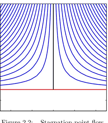
2.2.1 Stagnation-Point Flow
The potential-flow equations that mimic stagnation-point behavior can be represented in the
complex plane, where ζ =ξ+iη. The complex potential is given by the following equation:
F(ζ) = 1
2(ζ+β−i)
2 (2.3)
where the real and imaginary part represent the velocity potential and stream function
respec-tively.
The derivative of this complex potential in the ζ-plane gives the complex velocity, which
becomes:
F0(ζ) = dF
dζ = (ζ+β−i) (2.4)
Figure 2.2: Stagnation-point flow.
2.2.2 Flow Past a Parabola
The stagnation-point flow can be mapped onto the physical z-plane, using the transformation:
z= 1 2(ζ
2+ 1) (2.5)
The complex velocity in the z-plane can be obtained by applying the transformation from Eq.
2.5 to the complex velocity in theζ-plane:
F0(z) = dF
dz = dF
dζ
dz
dζ (2.6)
F0(z) = ζ+β−i
ζ (2.7)
F0(z) = 1 +β−i
ζ (2.8)
F0(z) = 1 +√β−i
2z−1 (2.9)
The real and imaginary part of the complex velocity in the z-plane are connected to the
velocity components in the x and y direction, respectively, given as u = Re{f(z)} and v =
Figure 2.3: Flow past a parabola.
system in which the parabola is written as Y =±√2X, where X and Y are non-dimensional
coordinates with respect to the radius of the parabola,r. That is,X =x/randY =y/r. Figure
2.3 shows the stagnation-point flow transformed into the flow past a parabola. Rewriting the
complex velocity in the X−Y coordinates gives:
F0(Z) = 1 + p β−i
2(X+iY)−1 (2.10)
F0(Z) = 1 +q β−i 2(Y22 +iY)−1
(2.11)
F0(Z) = 1 + √ β−i
Y2+ 2iY −1 (2.12)
F0(Z) = 1 +pβ−i
(Y +i)2 (2.13)
F0(Z) = 1 + β−i
(Y +i) (2.14)
Further algebraic manipulation to separate the the real and imaginary terms gives:
F0(Z) = Y(Y +β)
Y2+ 1 −i
Y +β
Therefore, the velocity components on the surface of the parabola are:
ux=
Y(Y +β)
Y2+ 1 (2.16)
uy =
Y +β
Y2+ 1 (2.17)
Substituting the dimensional coordinates back in the equation using X = x/r and Y = y/r,
the net velocity on the surface of the parabola can be written as:
U =
q
u2
x+u2y (2.18)
U = py+rβ
y2+r2 (2.19)
Further transforming the equation in terms of the x-coordinate usingy=±√2rx gives:
U = ±
√
2rx+rβ
√
2rx+r2 (2.20)
U = √ x± √ rβ √ 2 p
x+r2 (2.21)
For the freestream velocityU∞, this expression is equal to the equation given by van Dyke as :
U U∞
=
√
x±a0
p
x+r2 (2.22)
The positive sign and negative sign refer to the upper and lower surface, respectively.
Substi-tutinga0=βpr/2, The final expression used in this research for the velocity on the surface of a parabola near the leading edge is:
U U∞
= A(
√
x±a0)
p
x+r2 (2.23)
where A is a multiplicative factor, of order one, which relates the flow on the parabola to
parameter also compensates for viscous effects during the nonlinear regression process discussed
in Chapter 3.
2.3
Aerodynamic Model
The aerodynamic model used in the LEFS algorithm is built on the equations of flow past a
parabola as derived in the previous section. The final expression for the surface velocity shown
in Equation 2.23 can be converted to the coefficient of pressure. Using Bernoulli’s equation, the
difference between the surface pressure and the known freestream static pressure can be written
as:
P −P∞=
1 2ρU
2
∞
"
1−
U U∞
2#
(2.24)
On combining Eqs. 2.23 and 2.24, we obtain:
P−P∞=
1 2ρU
2
∞ 1−A2
(√x±a0)2
x+r/2
!
(2.25)
x y
−a′√2r
a′2
In Eq. 2.25, the freestream static pressure, P∞, and densityρ are assumed to be known
quan-tities, and the parabola nose radius,r, and slope, λ, are the known geometry parameters based
on the parabola-airfoil matching, which is explained in Chapter 3. Eq. 2.25 is expressed for a
symmetric parabola in the parabola frame of reference as depicted in Fig. 2.4. Hence, for the
case of a cambered airfoil, the coordinates in this equation are transformed to the airfoil frame
of reference based on the inclination of the defined parabola that appropriately fits the airfoil.
0 0.2 0.4 0.6 0.8 −2
−1
0
1
x/c C p
Airfoil Parabola
(a) Angle of attack = 5 deg.
0 0.2 0.4 0.6 0.8 −2
−1.5
−1
−0.5
0
0.5
1
x/c C p
Airfoil Parabola
(b) Angle of attack = -5 deg.
Figure 2.5: A comparison of the pressure distribution on a cambered S809 airfoil obtained from XFOIL with the pressure distribution over a parabola obtained from Eq. 2.25. Here,r andλin the equations are estimated by generating the parabolic curve based on the leading-edge region of S809 airfoil, as discussed in Chapter 3.
To illustrate the application of this analytical model, the pressure distribution over a
parabola calculated using the above equation is compared with the pressures over an airfoil
obtained using the XFOIL code in Fig. 2.5. The flow behavior over a parabola accurately
mim-ics that over an airfoil in a region in proximity to the stagnation-point location, which lies on
the lower surface for the α = 5◦ and on the upper surface forα =−5◦ on the upper surface.
Hence, the pressure distribution over the parabola can be inversely used to solve for the
consideration. Five pressures were deemed sufficient to successfully perform this operation and
estimate the relevant flow characteristics. The following chapter illustrates the methodology
Chapter 3
Methodology
This chapter presents the methodology adopted to deduce the sectional aerodynamic parameters
from the pressures measured near the leading edge of the airfoil. The equation for flow past a
parabola, discussed in Chapter 2, serves as the fundamental aerodynamic model used in the
LEFS technique. In addition, there are critical steps involved in the LEFS algorithm that are
integral to successfully solving the aerodynamic model. The approach adopted for fitting the
parabola to the airfoil leading-edge is presented in Section 3.1 and the nonlinear regression
method is discussed in Section 3.3. Finally, the process of converting the LEFS output into
relevant aerodynamic quantities is explained in Sec. 3.4.
3.1
Parabola-Airfoil Matching
The LEFS algorithm exploits the parabolic nature of the airfoil geometry in the proximity of the
leading edge. The airfoil leading edge radius,r, and the initial slope of the airfoil camberline,λ,
are the parameters required to generate the parabolic curve that fits the leading-edge region of
the airfoil, according to van Dyke [34]. However, the flow solution in Equation 2.25 based on this
parabola is valid only in extreme proximity to the leading edge of the airfoil. In practical
appli-cations, such limited space is insufficient for the installation of sufficient pressure taps/sensors in
in the initial step using a curve-fit approach, that matches the airfoil leading-edge coordinates
with the equation of a parabola given in Equation 3.1 until 5% of the airfoil chord.
Conse-quently, new values of the parameters r and λ are determined based on this parabola-airfoil
matching that make the solution for flow past a parabola (based on new r and λ) acceptable
till about 5% of the chord.
y=±√2rx+λx (3.1)
3.1.1 Symmetric Airfoil
For a symmetric airfoil, the quantityλ(in Equation 3.1) drops out and the equation is reduced
to an elementary form, y = ±√2rx. This also implies that, at α = 0 the stagnation point
coincides with the leading edge on the airfoil and the parabola. The equation of a symmetric
parabola is solved with the known airfoil coordinates in the leading-edge region (until 5% of the
chord) via a curve-fitting approach, to estimate a new leading-edge radius. The new value ofris
used in the aerodynamic model in Eq. 2.25 to render the solution acceptable for a considerable
parabolic envelope on the airfoil nose. Figure 3.1 shows the parabolic profile generated using
the new r for a symmetric NACA 0012 airfoil.
3.1.2 Cambered Airfoil
For a cambered airfoil, an ideal angle of attack is defined as the angle of attack at which the
stagnation point coincides with the leading edge of the airfoil. To define a parabolic profile that
models the nose of the airfoil, it is crucial to ensure that the stagnation-point location on the
leading-edge of the airfoil closely matches with that on the constructed parabola. The αideal
for the airfoil is estimated using inviscid velocity distributions obtained from the airfoil design
and analysis code, XFOIL[51]. The slope of αideal determines the new inclination, λ, for the
parabola. The leading-edge radius of the parabola that fits the airfoil nose reasonably well is
estimated by following a trivial curve-fit approach as adopted for the case of a symmetric airfoil.
0 0.02 0.04 0.06 0.08 0.1 −0.05
0 0.05
y r= 0.0135
x
NACA0012 Parabola Parabola axis
(a) Leading-edge region.
0 0.1 0.2 0.3 0.4 0.5 0.6 0.7 0.8 0.9 1 −0.1
0 0.1
y
x
NACA0012 Parabola
(b) Full airfoil.
Figure 3.1: Leading-edge parabola fit for a symmetric NACA 0012 airfoil.
1. Start with an initial guess value of r and generate a symmetric parabola.
2. Rotate this parabola byθ=αideal about a point on the camberline of the airfoil with the
x-coordinate equal tor.
3. Compare the coordinates of the rotated parabola with the airfoil nose-region till 5% of
the chord by evaluating a cumulative error function, δ = N
X
i=1
(ypi −yia)2 (superscripts p
and arepresent the parabola and airfoil respectively).
4. Determine the value of r iteratively till the δ is minimized.
Figure 3.2 compares the parabola-fit for a cambered airfoil. The new value ofrdetermined here
is used directly in Eq. 2.25. The aerodynamic model in LEFS is solved in a frame of reference
attached to the axis of the parabola. Therefore, for a cambered airfoil the pressure tap locations
0 0.02 0.04 0.06 0.08 0.1 −0.05
0 0.05
y rλ= 0.0136
=−0.0101
x S809 Parabola Parabola axis Point of rotation
(a) Leading-edge region.
0 0.1 0.2 0.3 0.4 0.5 0.6 0.7 0.8 0.9 1 −0.1
−0.05 0 0.05 0.1 0.15
y
x
S809 Parabola
(b) Full airfoil.
Figure 3.2: Leading-edge parabola fit for a cambered S809 airfoil.
the airfoil nose.
3.2
Selection of pressure-port locations
The aerodynamic model presented in Section 2.3 solves for three output parameters, U∞, A,
and a. A notable approximation in this simplified model is that it is derived from the inviscid
equations of flow past a parabola. As a result, the direct input of all the five measured pressure
values in the algorithm for any aerodynamic orientation might not yield accurate results, which
is evident by observing the pressure distribution over the parabola shown in Figure A.7 in
Chapter 2. The prime reason for utilizing five pressure data points is to be able to envelope
the leading-edge region and select pressure data points near the stagnation-point location. At
flow on the upper surface from that on the lower surface. Since the boundary-layer formation
commences from this point onwards, the boundary layer is relatively thin in this region, thereby
exhibiting close resemblance to the inviscid pressures in the vicinity of the stagnation point. The
pressure difference between the first pressure ports aft of the leading edge on the upper and the
lower surface provides a reliable indication of whether the airfoil is operating at a positive or a
negative angle of attack. Based on that information the pressure-tap information corresponding
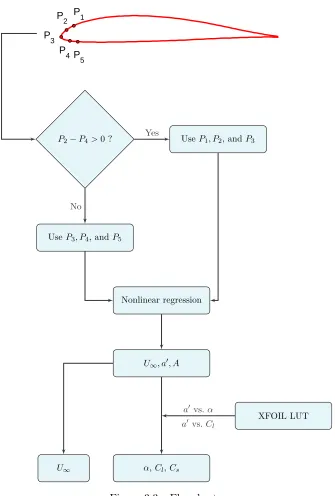
to the location of the stagnation point is used as depicted in the flow chart shown in Figure 3.3.
3.3
Nonlinear Regression
The aerodynamic model, for knownP∞,randλ, is provided in Equation 2.25. The aerodynamic
model can be represented byF, which is a function of the location of theith pressure port (xi),
a0,A, andU∞. If the measured pressure at theithpressure port isPi, then the error,i, is defined
as the difference between the pressure measured by the sensor and the pressure estimated from
the functionF, given as:
i=Pi−F(xi, a0, U∞, A) (3.2)
The sum of the errors for alln pressure ports under consideration is:
S = n
X
i=1
2i (3.3)
The algorithm minimizes this residual functionS to solve for the quantitiesa0 andU∞.
Numer-ous optimization techniques are available that use iterative procedures to solve such regression
problems. The current procedure uses the nonlinear least-squares function (lsqnonlin) from the
optimization toolbox in MATLAB to estimate the aerodynamic variables. This function uses
the trust-region-reflective method for the non-linear curve fitting operation, which is based on
P
1
P
2
P
3
P
4P 5
P2−P4>0 ? UseP1, P2, andP3
UseP3, P4, andP5
Nonlinear regression
U∞, a0, A
XFOIL LUT
α,Cl,Cs
U∞
Yes
No
a0vs.α
a0vs.Cl
Figure 3.3: Flowchart.
3.3.1 Trust-Region Reflective Method
Iterative optimization techniques can be broadly studied under two categories: line-search
and then advance along this path to solve for a better solution, which is utilized in the following
iteration to identify the new search direction. Trust-region algorithms construct an approximate
model near the current best point and then solve the model to yield a better solution. The
pro-cess is repeated until the final best solution is achieved. However, the approximate models are
only valid in a “trust” region in the vicinity of the current iterate. Generally, a merit function
is devised to track the performance of the model in the trust region. Consequently, it can limit
or enlarge the size of the trust region. A review of different trust-region algorithms is presented
by Yuan. [53]. The aproach used in thelsqnonlin function in MATLAB is developed by forming
a model with an appropriate quadratic function and scaling matrix. In addition to greater
re-liability and robustness, these methods have strong convergence properties and the capability
to effectively handle bound constraints [54].
3.4
Determining Aerodynamic Parameters
The methodology presented in the previous sections provides a step-by-step description of the
LEFS technique. The steps are summarized with the aid of a flowchart shown in Figure 3.3.
Five pressure values sensed on the airfoil surface in the neighborhood of the leading-edge are
used as inputs to the LEFS algorithm to return U,a, andAby employing nonlinear regression
techniques. The local freesteam dynamic pressure or velocity is obtained directly from the
current approach. The analytical function derived for velocity distribution using the parabola
model (Eq. 2.23) is differentiable and can be conveniently analyzed to obtain the local minimum
and maximum values. The minimum value of the function in terms ofarelates to the
stagnation-point location on the airfoil surface as:
xstag =a02 (3.4)
ystag =−a0
√
Similarly, the pressure-peak location can be estimated from the maximum value of the velocity
distribution as:
xpeak =
r2
4a02 (3.6)
substituting this value in the Cp distribution over a parabola results in:
Cppeak = 1−A2
(r+ 2a02)
r (3.7)
In addition to capturing the pressure behavior in the leading-edge region of the airfoil, the
parameters A and a0 can be successfully used to extract additional aerodynamic information,
such as the local angle of attack and lift coefficient. Two approaches were explored in this
research to relate the LEFS output parameters to the local flow-field characteristics. The first
approach utilizes asymptotic matching to directly relate a0 and A toα, while the second
ap-proach relies on the stored look-up tables previously-developed using low-order simulation or
CFD data. A detailed explanation of the two approaches is presented in the following
subsec-tions.
3.4.1 Direct Approach
Asymptotic matching is employed to derive a direct relationship between a, A and the local
angle of attack. The process exploits the fact that the flow around an airfoil involves two
disparate lengths, which means that the flow-field around the airfoil can be divided into two
regimes based on the length scales. The inner region is defined near the nose of the airfoil,
x ∼O(r), where the flow is characterized by extreme velocity changes due to the presence of
the stagnation-point and the suction peak and the length scale is governed by the leading-edge
radius,r. The outer region is defined around the rest of the airfoil where the flow is dominated
by classical thin airfoil theory. For viscous flows, the boundary layer also plays a significant
role in the interaction between the two regions because the boundary layer formation initiates
edge. However, in this analysis only the inviscid flow-field is matched in the near-nose region
and the rest of the airfoil. Asymptotic theory is used to match the solutions in an overlapping
domain. The existence of such an intermediate overlapping region implies that the inner limit
of the outer region should agree with the outer limit of the inner region, to appropriate orders
of magnitude [55].
The formulation for matching the inner and outer flow regions has been presented by
re-searchers while investigating the problem of leading-edge stall of an airfoil. Rusak and
Mor-ris [56] performed the matching which accounted for the interactions between the near-wall
viscous flow and the outer inviscid flow. Their analysis resulted in a model (simplified)
prob-lem of a uniform, compressible, steady stream past a semi-infinite parabola with a far-field
circulation governed by a parameter that is related by the asymptotic matching to the angle of
attack, nose radius of curvature, the airfoil camber and the flow Mach number. Tuck [57] had
developed a similar matching approach but used the exact potential flow around the nose of
the airfoil (replaced by a parabola) and matched in the far field with the thin-airfoil solution
resulting in an expression relating the parameter β to the angle of attack, nose radius and the
airfoil chord. This parameter is equivalent to the parameterβ used in deriving the equation of
flow past a parabola from stagnation-point flow in Section 2.2.2. In terms of the notation used
in the current research,β =a0Ap2/r.
In the current formulation, Tuck’s approach for matching the solution on the parabola and
the airfoil is followed. The outer matching provides a solution for the thin-airfoil theory in the
inner limits, x → 0, while the inner matching provides a result for non-dimensional parabola
solution in the outer limits ,X→ ∞. Similar-order terms from the limiting values of the inner
Outer Matching
The upper and the lower surface of an airfoil can be written in terms of the camber function,
fc, and the thickness function, ft, as:
y=fc(x)±ft(x), 0≤x≤c, (3.8)
For a small angle of attack, the rotated airfoil profile with respect to the freestream velocity
takes the form:
y=−αx+fc(x)±ft(x), 0≤x≤c, (3.9)
The fluid velocity is∇(U x+φ), whereφis the disturbance velocity potential due to the airfoil. It
follows that the solution of Laplace’s equation subject to the relevant boundary conditions, and
the Kutta condition at the trailing edge, results in the airfoil streamwise disturbance velocity
as:
u=φx=±U α
c−x x
12
±U
π
c−x x
12 Z c
0
fc0(ξ)
x−ξ
ξ c−ξ
12
dξ+U
π
Z c
0
ft0(ξ)
x−ξdξ (3.10)
The behavior of this thin airfoil solution near the leading edge can be simplified to:
ux→ ±U α
c x 1 2 (3.11) Inner Matching
Using the complex velocity for the parabola as derived in Section 2.2.2, theX-wise disturbance
velocity can be obtained. The non-dimensional complex velocity for a parabola flow is:
F0(Z) = 1 + β−i
For|Z| → ∞,
F0(Z)→1 +β−i
Y (3.13)
TheX-wise disturbance velocity is the difference between the freesteam velocity and the velocity
on the parabola as |Z| → ∞. This result is equal to ±β(2X)−12 . This disturbance velocity is
derived for the non-dimensional potentialF(Z). However, for the parabola problem, the actual
complex potential is U AF(z). The disturbance velocity on the parabola up becomes :
ux→ ±U A
β√r
√
2x (3.14)
whereβ =
√
2a0
√
r . Hence, the expression in terms ofa
0 becomes:
ux → ±U A
a0
√
x (3.15)
Comparing the terms in Eq. 3.11 and Eq. 3.15 gives a relationship between the angle of
attack and the parabola parameters,a0 and A, as :
α= a
0A
√
c (3.16)
The matching produces an expression to estimate the angle of attack directly from the output
parameters of the LEFS algorithm, i.e. a0 and A. Further this result can be used with the
thin-airfoil theory expression for the airfoil lift coefficient, which is:
Cl= 2π(α−αol) (3.17)
Cl= 2π
a0A
√
c −α0l
(3.18)
thin-airfoil theory. Furthermore, suction-force near the leading edge can also be obtained from
the LEFS parameters. Leading-edge suction is caused by the stagnation point moving away
from the leading edge to some other location when the airfoil is at an angle of attack. The
flow stops at the stagnation point and must travel around the airfoil’s leading edge towards the
other surface. The importance of this force coefficient is better understood from the perspective
of unsteady aerodynamics. The derivation for the suction-force coefficient, Cs, is presented in
detail in Sec. 4.3.1. The expression relatingCs toa0 and A takes the form:
Cs= 2π
a0A
√
c −
1
π
Z π
0
dfc
dx(θ)dθ
2
(3.19)
wherefc is the camberline of the airfoil and θ is a transformation variable related tox as:
θ= cos−1
1− 2x
c
(3.20)
The inner-outer matching used in the current formulation is applicable solely to thin airfoil
with thickness less than 15% of the chord. The inaccuracy for thick airfoils caused due to
this limitation is demonstrated in Chapter 4, where the direct approach is assessed for thicker
airfoil. Hence, a look-up table approach is proposed for extending the application of the LEFS
algorithm to airfoils where thickness effects are more pronounced.
3.4.2 Look-up Table Approach
Due to the complexity associated with accommodating the thickness effects in the direct
ap-proach, a look-up table approach is adopted in the LEFS algorithm to estimate αand Cl from
a0. The parameter a0, obtained from solving the aerodynamic model, strongly relates to the
angle of attack and can be effectively used to generate the look-up tables. XFOIL is used to
compute pressure data for several Reynolds numbers for a range of angles of attack
encom-passing both positive and negative stall angles. Five pressure values, extracted from the data,
are generated with one having the α vs. a0 values and the other having the α vs. Cl data.
For any airfoil under consideration, such tables can be generated from computational data and
integrated into the algorithm prior to the application. In real-time operation, the flow velocity
solved from the aerodynamic model at any instant is translated to the local Reynolds number,
which is then used along with a0 to extract the angle of attack and lift coefficient from the
tables. The effectiveness of the LEFS technique is evaluated under different flow conditions,
Chapter 4
Applications and Results
This chapter presents the application of the LEFS approach to different flow scenarios to
char-acterize the performance of the LEFS technique. Computational simulations and experimental
test data were used for various airfoils exhibiting different aerodynamic behavior. Section 4.1
shows the results of the LEFS algorithm applied to steady flow conditions. The capability of
the technique for the identification of airfoil stall and the estimation of aerodynamic parameters
beyond stall is explored in Sec. 4.2. Unsteady aerodynamic flows are investigated in Sec. 4.3
with the objective of capturing the signatures associated with the formation of leading-edge
vortices using the outputs of the LEFS approach. Finally, the ability of the current approach
to deduce the local sectional aerodynamic quantities for different sections of a rotating blade is
tested and the results are presented in Sec. 4.4.
In all the investigations, five pressure measurements and their locations are extracted from
the computational or experimental test data and this information is processed through the
LEFS algorithm to determine the sectional characteristics like angle of attack, lift-coefficient,
and freestream velocity, and the results are compared with the corresponding actual values
4.1
Steady Flow (Pre-Stall)
The LEFS algorithm was evaluated for steady flow conditions. Computational data available
from previous research studies in the NCSU Applied Aerodynamics Research Lab was utilized
for this study. Experimental data was gathered from National Renewable Energy Laboratory
(NREL) wind-tunnel test campaigns conducted at the Ohio State University wind tunnel.
4.1.1 CFD Test Cases
NCSU’s REACTMB-INS code was used for CFD calculations and the details of the
computa-tions and validation studies are discussed in Ref. [58]. Steady flow calculacomputa-tions over the airfoil
surface were performed for a range of angles of attack and the surface pressure data was
post-processed to extract the pressure information at five discrete locations near the leading-edge.
The five pressure values along with the respective locations on the surface are given as input
to the LEFS algorithm, and the aerodynamic parameters are determined as described in
Sec-tion 3.4. The test cases were evaluated for different airfoils: NACA 0012, SD 7003, and NACA
23012 at a Reynolds number of 3 million. The locations at which the pressures were extracted
from the CFD data for all the three airfoils are tabulated in Table 4.1.
Table 4.1: Pressure port locations used to extract data for LEFS inputs from CFD data.
Airfoil Pressure locations (x/c)
NACA 0012 Lower surface: 3.5% and 5.0%, (12% thick) Upper surface: 3.5% and 5.0%,
and Leading Edge SD 7003 Lower surface: 1.0% and 5.0%, (8.5% thick) Upper surface: 0.5% and 5.0%
and Leading Edge NACA 23012 Lower surface: 1.0% and 4.5%,
(12% thick) Upper surface: 0.8% and 3.5% and Leading Edge