Macroscopic Models for Shape Memory Alloy Characterization and Design

(1)

Abstract

Massad, Jordan Elias. Macroscopic Models for Shape Memory Alloy Character-ization and Design. (Under the direction of Dr. Ralph C. Smith.)

(2)

issues pertinent to thin-film SMAs. Furthermore, the model admits a low-order formulation and has a small number of parameters which can be readily identified using attributes of measured data. We illustrate aspects of both models through comparison with experimental bulk and thin-film SMA data.

(3)

(4)

Jordan E. Massad, with the assistance of a registered nurse, first opened his eyes to

mathematics on May 20, 1976 at approximately 5:00 AM. Raised in Tulsa, Oklahoma by Joseph and Darlene Massad, his affinity towards mathematics developed early on. At 12 years old, he memorized over 100 digits of π to pass the time in programming class; to this day he can recite 58 digits at a moment’s notice. At the age of 14, he derived the rate law for radioactive decay in his chemistry class.

In 1998, he earned a Bachelor of Science degree in physics and mathematics at Worcester Polytechnic Institute in Worcester, Massachusetts. That same year, he embarked on an arduous journey toward applied mathematics master’s and doctoral degrees at North Carolina State University in Raleigh, North Carolina. He entered the Department of Mathematics under the U.S. Department of Education Graduate Assistance in Areas of National Need Fellowship in Scientific Computation. As part of the Industrial Applied Mathematics program in the Center for Research in Scientific Computation, he conducted research at The Boeing Company in Bellevue, Washington (1999) and at Sandia National Laboratories in Albuquerque, New Mexico (2001-2002). Ultimately, under the tutelage of Professor Ralph C. Smith, he focused his research on the modeling of shape memory alloys, with an emphasis on thin films for microelectromechanical systems. Following his retirement from academia, he will begin his professional career as a Senior Member of Technical Staff at Sandia National Laboratories.

(5)

Acknowledgments

I deeply appreciate the support from my family: my parents, Joseph and Darlene; my siblings Rob, Jolene, Joshua, Jodain, and Joslyn; and my grandparents, aunts, uncles, and innumerable cousins. I also appreciate the mental and culinary support from my extended Lebanese family in Raleigh, including the Haddad’s, Ishak’s, Mitri’s, and Saleh’s. Of the numerous graduate students I have had the pleasure to befriend, I especially appreciate my office mates in legendary HA208: Brian, Kathy, Kristy, Lea, Michele, Gail, Katie, Rachel, Nick, Matt, Julie, and Jill.

I sincerely appreciate my mathematical grandfather, Brother Bernadine Kuzmin-ski, for inspiring me to seek and engage the many challenges of advanced mathematics. I genuinely acknowledge Ralph for helping to steer me to NCSU and for supporting and putting me on a path of unbridled success and academic professionalism. I also thank the committee for raising insightful points regarding components of my research; by addressing these issues, both the presentation and content of my disserta-tion were improved. Addidisserta-tionally, I am grateful for the assistance from Dr. Seelecke’s students, Olaf Heintze and Jason Frautschi from the Department of Mechanical and Aerospace Engineering at NCSU. Moreover, I acknowledge Dr. Jim Redmond for providing me extremely rewarding experiences at Sandia National Laboratories.

I greatly appreciate those who provided me with experimental data and analysis: Dr. Borut Bundara at ETRA 33 in Ljubljana, Slovenija; Dr. Ken Gall from the

(6)

Fuji Matsuzaki and Hisashi Naito at the Structural Dynamics Lab within Nagoya University in Nagoya, Japan; Dr. Greg P. Carman, Jason Woolman, and Dr. K.P. Mohachandra from the Active Materials Laboratory at UCLA in Los Angeles, CA; and Dr. Akira Ishida from the Materials Engineering Laboratory at the National Institute for Materials Science in Tsukuba, Japan.

Finally, I acknowledge my sources of funding that helped provide the resources I needed to accomplish my degree: the National Science Foundation under the grant CMS-0099764; the Air Force Office of Scientific Research through grant AFOSR-F49620-01-1-0107; the U.S. Department of Education GAANN Fellowship in Scientific Computation; and Sandia National Laboratories.

(7)

List of Figures

1.1 Idealized hysteresis for superelasticity and the shape memory effect. . 2

1.2 A single crystal under uniaxial loading with three stable configurations. 3 3.1 A Landau free energy describing a crystallographic system with three equilibrium phases. . . 21

3.2 The equilibrium stress-strain model for increasing temperatures. . . . 25

5.1 The domain model for different temperatures. . . 38

5.2 Superelastic hysteresis simulation at T = 295 K. . . 39

5.3 The initial fit of the domain model compared to data. . . 41

5.4 The final fit of the domain model compared to data. . . 42

6.1 A piecewise quadratic Helmholtz free energy density. . . 51

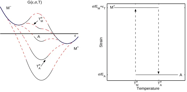
6.2 The specific Gibbs free energy at a fixed temperature T > T_M and varying stress. . . 52

6.3 The specific Gibbs free energy at a fixed stress and varying temperatures. 53 6.4 The non-dimensional chemical free energy for various ∆c≥0. . . 56

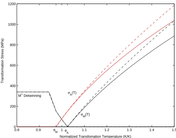
6.5 The phase transformation stresses and transformation temperatures normalized by T_eq. . . 59

(12)

low thermal energy. . . 65

6.7 The transition rates P_± and P_A_± for a fixed temperature T > T_A and varying stress. . . 66

6.8 The expectation strains as a function of stress (T > T_A) and temper-ature for low thermal energy. . . 68

6.9 Superelasticity (fixed T > T_A) and shape memory effect (fixed stress) hysteresis determined from the expected strain. . . 70

7.1 The log-normal probability density function compared with its normal counterpart. . . 78

8.1 Superelasticity at T_E = 358 K. . . 86

8.2 The temperature-dependence of the hysteresis. . . 87

8.3 Shape memory effect with a constant stress of 200 MPa. . . 88

8.4 The stress-dependence of thermal hysteresis. . . 88

8.5 Superelasticity and SME for different film thicknesses. . . 89

8.6 Joule heating of a thin-film SMA and cooling via forced convection. . 90

8.7 The time response of a 10 µm thin-film SMA. . . 91

9.1 The average local material response compared with the statistically homogenized macroscopic response. . . 93

9.2 Identification of material parameters using stress-strain hysteresis data. 94 9.3 Identification of material parameters using strain-temperature hystere-sis data. . . 96

9.4 The phase evolution model compared to stress-strain data for an SMA thin sheet. . . 99

(13)

9.5 The phase evolution model compared to thin-film SMA stress-strain data. . . 101 9.6 The phase evolution model compared to thin-film SMA SME data. . . 102

(14)

Introduction

1.1 Shape Memory Alloys

Shape memory alloys (SMAs) are metals that recover from up to 10% deformation via stress and temperature-induced phase transformations. SMAs undergo martensitic transformations, which are displacive transformations dominated by shear distortions of the crystal lattice. Transformations occur between two solid phases, called marten-site andaustenite. Distinguished by their crystallographic structures, martensite and austenite can have drastically different mechanical, thermal, electrical, optical, and acoustical material properties [81]. In general, martensite is the material phase that is stable at low temperatures relative to austenite, which is stable at high temperatures. The martensitic transformations between martensite and austenite enable SMAs to recover or “remember” shape by two different mechanisms. In both cases, austenite corresponds to the remembered shape. First,superelasticity describes shape memory via stress-induced phase transformations. At a fixed temperature where stress-free austenite is a stable phase, austenite transforms into martensite due to an applied load. Upon removing the load, the material reverts to austenite and the original shape

(15)

CHAPTER 1. INTRODUCTION 2

0

Temperature

Strain

Shape Memory Effect

0 0

Stress

Strain Superelasticity

Martensite

Austenite

Martensite

Austenite

Unload Load

Cool

Heat

Figure 1.1: Idealized hysteresis for superelasticity (fixed temperature) and the shape memory effect (fixed load).

is recovered. Secondly, theshape memory effect (SME) describes shape memory via temperature-induced transformations. In this case, deformed martensite transforms into austenite due to heating and shape memory is observed. Upon subsequent cooling, the SMA transforms back to martensite. If the SMA is stress-free upon cooling, then it will retain its recovered shape in the martensite phase by means of a process called self-accommodation. If the SMA is subjected to a load while cooling, then it will deform again as it reverts to martensite.

(16)

Figure 1.2: A single crystal under uniaxial loading with three stable configurations: austenite (A) and martensite variants (M±). The arrows indicate shearing and the associated shear strain is ε_s = tanθ.

When reheated to austenite, the transformation strain is recovered. As we illustrate in Parts I and II, the general stress-temperature-strain behavior of SMAs is ther-momechanically coupled. We refer the reader to [81] for details of shape memory mechanisms and other SMA material properties.

(17)

SMAs can be prepared as a single crystal, but they occur more naturally as poly-crystalline compounds. Asingle-crystal SMA refers to a SMA specimen that consists of unit cells of only one crystallographic orientation. Apolycrystalline SMA consists of many single-crystal grains with various orientations. The behavior of single-crystal SMAs differs from that of polycrystalline SMAs in several aspects. For example, single-crystal NiTi recovers from up to 10% tensile strains, depending on the crystal orientation, whereas polycrystalline NiTi typically recovers no more than 8% tensile strains [11]. We model aspects of both single-crystal and polycrystalline SMAs in Parts I and II.

1.2 Applications

The hysteresis exhibited by shape memory alloys enables the materials to achieve very high work densities, produce large recoverable deformations, and generate high stresses, which are ideal for a number of high performance applications. For example, medical and potential aeronautic and aerospace applications are being investigated to employ SMAs’ large deformation and large force capabilities [21, 53]. Additionally, SMAs exhibit a damping capacity much larger than that of a number of conventional materials. In this case, SMA hysteresis is being utilized to design earthquake and hurricane-proof civil structures [20, 91, 106, 118].

(18)

and, unlike bulk SMAs (wires, beams, etc.), their small mass and large surface-to-volume ratio allow fast cooling rates, potentially permitting switching frequencies on the order of 100 Hz [29, 72, 87].

Current microscale SMA applications include microgrippers [60], micropumps [120], and microcantilever switches [30, 50, 76]. Most of these applications rely on the one-way memory effect and require a biasing mechanism for full actuation. How-ever, microdevices using functionally graded films can achieve two-way, out-of-plane displacement with a smaller footprint than conventional micromechanisms [38, 39]. Superelastic NiTi thin films are being considered for high-strength surface coatings in MEMS devices, and they have potential for microscale mechanical energy storage devices, and vibration dampeners in microelectronics packaging [41, 46]. We refer the reader to [63] for a review of other thin-film SMA applications.

1.3 Modeling Approaches

To achieve the full potential of SMA actuators, it is necessary to develop models that characterize the nonlinearities and hysteresis inherent in the materials. Most models of hysteresis in SMAs are constitutive, aiming to predict the measured relationships among stress, temperature, and strain. We refer the reader to reviews and compar-isons of a number of models in [12, 17, 27, 35, 88] and particularly in [94], where computational considerations are addressed. SMA hysteresis models can be roughly categorized as being microscopic, mesoscopic, or macroscopic, depending on which material level they base their method of predicting constitutive behavior.

(19)

ferroelastic compounds. Understanding material dynamics at these fundamental lev-els can support efforts to design compounds with desired material properties. For example, Cast´an, et. al. [18] quantify interatomic energies and conduct lattice model simulations for some ferroelastic alloys. Given atomic composition and thermal treatment information, they are able to compute macroscopic elastic constants and martensite transition temperatures. Models of this nature are typically used for off-line simulations, and their solution requires techniques such as Monte Carlo methods that have a high computational cost.

Another class of mesoscopic models, traditionally referred to as micromechani-cal models, focuses specifically on developing local grain-level constitutive theories [25, 34, 83]. While operating at a fundamental level similar to that of the pre-viously mentioned theory, these models provide a more direct means of predicting observed constitutive behavior. Deriving macroscopic constitutive behavior from these theories for design applications necessitates additional procedures, such as the self-consistent averaging approaches in [34, 83]. Scaling these mesoscopic theories to macroscopic levels usually is computationally intensive; therefore, for macroscopic predictions, these models are generally not intended for on-line engineering nor con-trol applications. Recently, micromechanical models have been developed specifically for thin-film SMAs [6, 58].

(20)

constitu-tive relation. Similarly, Papenfuß and Seelecke [82, 95] predict thermomechanical behavior by modeling the evolution of martensite variant fractions, but by using a statistical thermodynamics description of thermally activated processes. Gabry and Lexcellent [32, 69] have developed similar models for thin-film SMAs.

Another macroscopic approach, based on phenomenological principles, is the Preisach model [114]. Originally developed for ferromagnetic hysteresis, Preisach models have been generalized and adapted to other physical systems, including SMAs [33, 44, 47, 64, 65, 74, 117]. In general, Preisach models are purely empirical and their implementation reduces to the identification of many mathematical parameters via numerous hysteresis experiments that may be unavailable in practice. To make Preisach models more tractable for SMA applications, there have been attempts to re-place or identify purely mathematical constructs with known or approximated physics. For example, Huo [47] incorporates Falk’s [22] macroscopic Landau-Ginzburg po-tential to account for first-order martensitic phase transformations. In addition, Lagoudas and Bhattacharyya [65] associate Preisach weighting functions with distri-butions of single-crystal orientations in polycrystalline SMAs.

(21)

(22)

The Domain Model

(23)

Chapter 2 Ferroelastic Materials

A ferroelastic material is one in which there is a mechanical switching between ori-entation states of its underlying crystal structure. The switching process, termed a ferroelastic phase transition, is a displacive structural phase transition that gives rise to an observable shape-change in the material. A measure of the crystal distortion is the spontaneous strain, analogous to the spontaneous magnetization and polarization respectively associated with ferromagnetic and ferroelectric transitions. Measure-ments of spontaneous strains during ferroelastic phase transitions show ferroelastic material behavior to be generally nonlinear, exhibiting temperature-dependent elas-tic hysteresis (e.g., see [92]). Shape memory alloys are a distinguishable class of ferroelastics.

Ferroelastic Domains

Ferroelastic domains are regions of ferroelastic crystals distinguished by different strain states of definite crystallographic orientation [92, 108]. Roytburd, who orig-inally formulated the more general concept of elastic domains, shows that domains form in ferroelastics to minimize internal elastic energies [90]. Accordingly,

(24)

lastic domains in SMAs correspond to stable martensite and austenite strain states. Ferroelastic domain walls are boundaries or transition regions where strains change gradually between adjacent domains. In fact, phase transformations in SMAs proceed with the motion of domain walls as discussed in [24, 93]. When a transformation occurs, domains exhibit spontaneous strains and their corresponding domain walls

translate. In addition to translating, domain walls can bend about pinning sites, which characterize material impurities, inclusions, or inhomogeneities that hinder domain wall movement [68, 93].

It is commonly accepted that domain wall motion in ferroelastic materials yields hysteretic macroscopic behavior. Mueller, et. al. indicate in [77] that nonlinear effects in ferroelastic crystals are related to the properties of ferroelastic domain walls pinned on defects, which de-pin above some stress level. Additionally, Jian and Way-man [54] observe domain wall motion in stressed single-crystal and polycrystalline LaNbO₄ ferroelastics. They argue that the nonlinear elastic material behavior and the observed shape memory effect result from domain wall motion, and they reason that polycrystalline grain boundaries, like pinning sites, limit wall mobility. Fur-thermore, Newnham [80] concludes that stress-induced movement of domain walls is a source of the hysteresis observed in ferroelastics, and Salje [92] claims that macro-scopic spontaneous strains resulting from martensitic transformations are strongly influenced by a crystal’s domain structure.

(25)

fer-CHAPTER 2. FERROELASTIC MATERIALS 12

roelastic hysteresis is caused by the pinning of phase boundaries on lattice defects, as ferromagnetic hysteresis can be caused by the pinning of ferromagnetic domain walls. Furthermore, like Salje [92], they identify a ferroelastic coercive stress anal-ogous to the coercive fields in ferromagnetic and ferroelectric hysteresis. However, as discussed in [42], ferroelastic domain walls are typically an order of magnitude thicker than ferromagnetic domain walls, so as in ferroelectrics, reversible wall effects in ferroelastics are expected to be more substantial.

Given the experimental results of [54, 89] and the strong comparisons to ferro-magnetic and ferroelectric domain theory, a ferroelastic domain theory may provide a viable means for describing the nonlinear constitutive behavior of SMAs.

The model we present focuses on predicting macroscopic constitutive behavior by considering mesoscopic (domain level) energy relations. We derive our model based on a domain model formulation first used to predict ferromagnetic hysteresis by Jiles and Atherton in [55] and subsequently extended to ferroelectric compounds in [99]. Previous work to employ these techniques for ferroelastic materials includes [73, 110]. We take this approach for three main reasons. First, this theory produces models with few parameters, most of which can be readily identified from measurements and all of which can be updated quickly. Second, the model formulation is of low-order and lends itself to control design; it has been implemented into control algorithms via inverse compensation [98]. Third, successful development of a domain model for hysteresis in ferroelastics could provide a crucial step towards developing a unified methodology for modeling hysteresis in ferroic materials [100].

(26)

formula-tion to predict temperature-dependent stress-strain hysteresis, but no comparison to data is provided. Likewise, Stoilov and Bhattacharyya [105] model SMA hysteresis by describing the evolution of phase fronts (domain walls) during transformation. Neither accounts for material defects nor treats partial stress-strain cycles.

(27)

Chapter 3 Nonlinear Stress-strain Law

In this chapter, we derive a stress-strain law to model the superelastic response of SMAs in thermodynamic equilibrium. Shape memory mechanisms in SMAs are caused by first-order martensitic phase transformations. Accordingly, by describing these structural phase transformations, we obtain an expression for the stress-strain material response. Our approach follows from energy methods used in the nonlinear theory of finite thermoelasticity, where the construction of a multiwell strain-energy function is used to characterize constitutive behavior [2]. Free energy expressions for SMAs have been developed through various approaches [2, 10]. We take a phe-nomenological approach based on the Landau theory of phase transitions, which has been shown to yield appropriate approximations for the free energies correspond-ing to ferroelastic phase transitions [92] and has been used for SMA modelcorrespond-ing in [13, 23, 26, 73, 92, 105, 110]. In addition to ferroelastics, the Landau theory has been successful in modeling transitions in ferroelectrics and ferromagnetics [22].

First, we summarize the Landau theory currently established for SMAs, and we quantify the free energy of a single crystal as a function of strain. Second, we adapt

(28)

the single-crystal energy function to accommodate bulk polycrystalline specimens under tensile loading. Third, we obtain a stress-strain law from the effective free energy equations of state. Our ultimate result is a thermodynamic equilibrium relation predicting relative macroscopic elongation due to an applied stress at a fixed temperature.

3.1 The Landau Free Energy

The Landau theory is a phenomenological theory that establishes the consistency of microscopic crystal characteristics, such as space-symmetry, with macroscopic quan-tities, such as elasticity. Using lattice dynamics, elasticity theory, and group theory, it aims to derive a system free energy based on the symmetry changes of a crystallo-graphic phase transformation. In constructing the free energy expression, the Landau theory defines two fundamental concepts: the order parameter and the Landau free energy.

(29)

stud-CHAPTER 3. NONLINEAR STRESS-STRAIN LAW 16

ies have shown that martensitic phase transitions areimproper, treating macroscopic transformation strain as a secondary effect coupled to the primary order parameter. The primary order parameter, which solely determines the symmetry-breaking mech-anism, instead is expressed in terms of normal mode components of lattice modulation wave vectors [8, 9, 86, 115]. In its group theoretical formulation, the Landau theory restricts the order parameter to a quantity that spans the irreducible representation driving the symmetry-breaking transition.

The Landau free energy is a thermodynamic expression determined by symmetry properties of the crystallographic phase transformation. It is in the form of a polyno-mial expansion whose terms are invariant functions under the symmetry operations of the high-symmetry space group. For general ferroelastics, the Landau free energy is a function of the order parameter and spontaneous strain

L(Q_i, ε_i) = L_Q(Q_i) +L_ε(ε_i) +L_Qε(Q_i, ε_i), (3.1)

where L_Q is the expansion of the order parameter components Q_i, L_ε is the elastic energy expressed in terms of spontaneous strain componentsε_i (Voigt notation), and

(30)

sixth-order, the order parameter expansion invariant with respect to the cubic symmetry group O_h is

L_Q(Q_i) = β0 2I1+

β₁

4I2+

β₂

4I

2 1 +

β₃

6 I

3 1 +

β₄

6I1I2+

β₅

6I

2

3, (3.2)

where

I₁ =¡Q2₁+Q₂2+Q2₃¢, I₂ =¡Q4₁+Q4₂+Q4₃¢, I₃ =Q₁Q₂Q₃, (3.3)

for a three-component order parameter. In general, the energy coefficients β_i are temperature-dependent. The standard assumption in the Landau theory is that only the coefficient of the quadratic term depends on temperature and that it is propor-tional to (T −T₀), where T is the system temperature andT₀ is the critical tempera-ture of the phase transition, analogous to the Curie temperatempera-ture for ferroelectrics and ferromagnetics. This assumption, motivated by specific entropy and enthalpy con-siderations in [92], guarantees that the high-symmetry phase corresponds to a stable, stress-freehigh-temperature phase forT > T₀. Evidence for temperature-dependence in other coefficients is reported in [26, 113] for specific ferroic compounds. In (3.2), the Landau free energy accounts for transformations to and among four distinct low-symmetry phases. (An expansion to twelfth-order accounts for a maximum of eight phases.) By considering only those transformations and phases pertinent to the first-order B2-B190 transformation, the form of (3.2) simplifies to

L_Q(Q) = b2(T −T0)

2 Q

2₊b4

4Q

4₊ b6

6Q

6_, _(3.4)

(31)

Simpli-CHAPTER 3. NONLINEAR STRESS-STRAIN LAW 18

fication and reduction of general expansions is discussed in [92, 109]. We note that with b₂, b₆ > 0 and b₄ < 0, (3.4) is the minimum-order order parameter expansion that describes the first-order phase transition under the symmetry constraints. In the Landau theory, typically one uses the expansion of lowest-order to describe a phase transition with as simple a model as possible.

The elastic and coupling energies are left to be defined. Using standard Voigt notation, we take the symmetry-obeying elastic energy expansion

L_ε(ε_i) = 1 2

6 X

i,j=1

(c_ijε_iε_j) + 1 2

6 X

i,j=1

(c_ijklε_iε_jε_kε_l), (3.5)

where c_ij and c_ijkl are second-order and fourth-order elastic coefficients, respectively. A thermodynamic description of high-order elastic coefficients is provided in [14], and [103, 104] describe methods for measuring those of single crystals. Symmetry of the Landau free energy restricts terms of the order parameter-strain coupling energy to linear combinations ofQn_iεm_i , with integers m > n >0. Conserving the symmetry of the improper phase transition, we take a biquadratic coupling

L_Qε(Q, ε_i) = 1 2Q

2 X6

i,j=1

d_ijε_iε_j (3.6)

with a scalar order parameter and the constant coupling coefficientsd_ij. Refer to [92] for details on other coupling scenarios and measurements of the coupling coefficients. The Pm3mto P2₁/msymmetry breaking in NiTi restricts the spontaneous strain tensor components to four nonzero shear strains [92]. For a one-dimensional model, we consider a single nonzero shear component ε_s, which yields

L_ε(ε_s) = css 2 ε

2

s+

c_ssss

4 ε

4

(32)

and

L_Qε(Q, ε_s) = dss 2 Q

2_ε2

s.

Therefore the reduced Landau free energy in one spatial dimension is

L(Q, ε_s) = b2(T −T0)

2 Q

2 ₊b4

4Q

4₊ b6

6Q

6₊ css 2 ε 2 s+ c_ssss 4 ε 4 s+ d_ss 2 Q

2_ε2

s. (3.7)

Similar to techniques employed in [86, 92, 109, 110], we obtain a free-energy function solely in terms of strain by enforcing the stress-free equilibrium conditions

∂L

∂Q = 0 and ∂L ∂ε_s = 0,

which yields the relations

Q¡b₂(T −T₀) +b₄Q2+b₆Q4+d_ssε2_s¢= 0 (3.8)

ε_s¡c_ss+c_ssssε_s2 +d_ssQ2¢= 0. (3.9)

By construction, vanishing Qcorresponds to the high-temperature/symmetry phase, which we associate with zero deformation (austenite). Therefore, taking ε_s 6= 0 in (3.9) yields

Q2 =−css+cssssε

2

s

d_ss .

Then (3.8) implies

·

b₂(T −T₀)−b4css

d_ss + b₆c2_ss

d2_ss ¸

+

µ

d_ss− b4cssss d_ss + 2

b₆c_ssc_ssss d2_ss

¶ ε2_s+ +b6c

2

ssss

d2_ss ε 4

(33)

CHAPTER 3. NONLINEAR STRESS-STRAIN LAW 20

With a factor of ε_s, we take (3.10) as the equilibrium condition for an effective free energy in terms of shear strain

L_e(ε_s) = a s

6

6ε

6

s−

as₄

4ε

4

s+

as₂

2 (T −Tc)ε

2

s, (3.11)

with effective parameters

T_c =T₀+css(b4dss−b6css)

b₂d2_ss , a

s

2 =b2, as₄ = cssss(b4dss−2b6css)

d2_ss −dss, a

s

6 =

b₆c2_ssss d2_ss .

Provided T_c, as

2, as4, as6 > 0, (3.11) maintains the overall equilibrium behavior

es-tablished by symmetry in (3.4). Including higher-order nonlinear elastic terms in (3.5) results in an effective Landau free energy of higher-order. While a similar effect may be realized by increasing the order of the order parameter expansion, only the lowest-order expansion in (3.4) is necessary to guarantee a first-order transition to the monoclinic phase. As for the coupling energy, there lacks evidence that termsQn_εm i form+n >4 contribute significant amounts of energy in ferroelastic compounds [92]. Based on these arguments, we use an extension to (3.11)

Lm_e (ε_s) = m X j=3 µ as 2j 2j ¶

ε2_sj −a

s 4 4 ε 4 s+ as 2

2 (T −Tc)ε

2

s (3.12)

for m ≥ 3 odd, which we take to reflect higher-order elastic nonlinearities in the material. For constants as

(34)

L_e

ε_s

T = T c

T < T c

0

T >> T c

Figure 3.1: A Landau free energy (3.11) describing a crystallographic system with three equilibrium phases.

(35)

3.2 Effective Gibbs Free Energy

The Landau theory provides us with a free energy expression in terms of shear strain for a single crystal. The expression (3.12) corresponds to the reference Helmholtz free energy density at a fixed temperature T. Including the effects of an external field, we get the associated Gibbs free energy density

G_s(ε_s;σ_s) = m X j=3 µ as 2j 2j ¶

ε2_sj − a

s 4 4ε 4 s+ as 2

2 (T −Tc)ε

2

s−σsεs, (3.13)

whereσ_s is the shear component of stress conjugate toε_s. Resolved from the applied axial stress σ, the shear stress has the form

σ_s =σsinφcosθ, (3.14)

whereφis the angle between the habit plane and stress axis, andθis the angle between the shear direction and the stress axis [15, 43]. Similarly, the axial (engineering) strain

ε and the shear strain satisfy

ε =ε_ssinφcosφ. (3.15)

In our current formulation, we assume the habit plane and shear direction are identical so thatφ =θ. We refer the reader to micromechanical theories in [15, 36, 43] where this restriction is relaxed and shear orientations are calculated for specific crystal systems. Therefore, for a given orientation φ, (3.13) has the form

G_φ(ε;σ) = m

X

j=3

Ã aφ₂_j

2j !

ε2j −a

φ

4

4 ε

4₊aφ2

2 (T −Tc)ε

(36)

where

aφ₂_j =

µ

2 sin(2φ)

¶₂j

as₂_j, φ∈ ³

0,π

2

´

. (3.17)

For a bulk polycrystalline material with many grains of different orientations, we get an effective, macroscopic free energy by integrating over φ [23, 82] to obtain

G(ε;σ) =

Z _π/₂

0

G_φ(ε;σ)f(φ)dφ

= m

X

j=3

a₂_j

2j ε

2j₋ a4 4ε

4₊ a2

2 (T −Tc)ε

2₋_σε, _(3.18)

where

a₂_j =

Z _π/₂

0

aφ₂_jf(φ)dφ. (3.19)

Here, f(φ) represents a scaled statistical distribution of single-crystal orientations. The formulation of effective coefficients a₂_j in (3.19) is well defined, despite the sin-gularities in the integrands at φ = 0 and π/2. At these orientations, the applied stress has no shear component and ε_s = 0. Ultimately, the macroscopic free energy (3.18) differs from (3.13) only in the scaling of its terms.

3.3 Stress-Strain Equations

We derive a stress-strain law from (3.18) by employing equilibrium principles. The equilibrium state of the material is the strain value that yields a minimum Gibbs free energy given a stress σ at fixed temperature T. The stable equilibrium states (ε_an, σ, T) must satisfy the conditions

∂G ∂ε

¯¯ ¯¯

εan,σ,T

= 0 and ∂

2_G

∂ε2 ¯¯ ¯¯

εan,σ,T

(37)

Evaluating the conditions yields m

X

j=3

a₂_jε2_anj−1−a₄ε_an3 +a₂(T −T_c)ε_an =σ (3.21)

subject to

m

X

j=3

(2j −1)a₂_jε2_anj−2−3a₄ε2_an+a₂(T −T_c)>0, (3.22)

where ε_an is the strain at equilibrium.

(38)

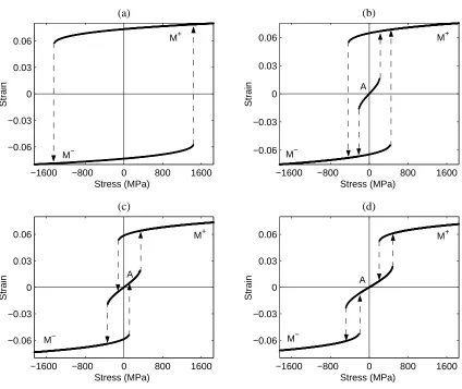
−1600 −800 0 800 1600 −0.06 −0.03 0 0.03 0.06 Stress (MPa) Strain (a)

−1600 −800 0 800 1600

−0.06 −0.03 0 0.03 0.06 Stress (MPa) Strain (b)

−1600 −800 0 800 1600

−0.06 −0.03 0 0.03 0.06 Stress (MPa) Strain (c)

−1600 −800 0 800 1600

−0.06 −0.03 0 0.03 0.06 Stress (MPa) Strain (d) M−

M+ M+

M− M−

M−

A

(39)

Chapter 4 The Domain Wall Model

The Landau-based constitutive theory of lattice-level behavior suggests that a ma-terial responds discontinuously when brought across a transformation point. The equilibrium relation (3.21) derived from the Landau free energy also predicts dis-continuous behavior at the macroscopic level, however, which is not an observed phenomenon [81, 96, 110]. Solutions to this dilemma have been to use a Landau-Ginzburg free energy to augment the Landau potential with strain-gradient terms. The result of this approach is an expression for the geometry and motion of phase boundaries as transverse shock waves in the absence of material dislocations [24, 105]. Realistically, ferroelastics contain material inclusions and other inhomogeneities that are manifested as an internal friction that inhibits phase boundary motion and that dissipates elastic energy. To account for impurities and energy losses, we treat the macroscopic measured strainεas a result of crystal domain reorientations impeded by lattice defects. We call the strain that would be measured in the absence of material inhomogeneities the anhysteretic strain, ε_an. By definition, the anhysteretic quan-tity in the Jiles-Atherton model for ferromagnetic compounds represents the system

(40)

response that would be obtained in the absence of hysteresis effects. In [55, 99, 101], each point on an anhysteretic curve corresponds to a global energy minimum for a given external field. Accordingly, this interpretation restricts the single-valued an-hysteretic strain to lie on only the absolutely stable portions of the equilibrium strain curves illustrated in Figure 3.2. The absolutely stable states represent the Maxwell states of an elastic body [2, 23, 78]. As in [110], we interpret the anhysteretic strain in ferroelastics to be identical to the multivalued equilibrium strain in (3.21), which reflects both absolutely stable and metastable energy states.

In addition to ε_an, we identify two macroscopic strains that are brought about by domain wall motion. We denote the irreversible strain ε_ir as that which manifests from domain wall translation across pinning sites. We denote the reversible strain

ε_re as that which manifests from domain wall bending about pinning sites. The total macroscopic strain ε is the sum of the two. In this chapter, we quantify irreversible and reversible strains in terms ofε_an to predict measured bulk strain.

4.1 Domain Wall Pinning

(41)

CHAPTER 4. THE DOMAIN WALL MODEL 28

stress σβ(T), where β ∈ {∓,−A, A+} denotes the switch from M− to M+, M− to

A, and A to M+, respectively. The strain εtr_β (T) is the spontaneous transformation strain accompanying the domain switching, illustrated by the jumps in Figure 3.2, which is essentially the strain manifested by wall translation. For an applied stress

σ ≥σ_β(T) at temperature T,

Eβ(T) =

Z

σ(ε)dε=σ_β(T)εtr_β (T)

is the energy generated per unit volume in translating a singleβ-domain wall. There-fore, the total energy per unit volume is

E(T) =X β

Eβ(T). (4.1)

We reformulate (4.1) as

E(T) = ¯σ(T)X β

εtr_β (T) (4.2)

where

¯

σ(T) =

P

β_Pσβ(T)εtrβ (T) βεtrβ (T)

. (4.3)

Following Jiles and Atherton, we assume that the energy required to move a domain wall across a pinning site is proportional to the energy of unimpeded domain wall movement. Lettingn_β denote the number density of pinning sites at aβ-domain wall, we approximate the pinning energy density by

Epin(T) =Cσ¯(T)

X

β

(42)

where C is a proportionality factor. One can establish a constant C in terms of quantities at a fixed temperature. For T =T_c, (4.4) simplifies to

Epin(Tc) = Cσ∓(Tc)n∓εtr∓(Tc). (4.5)

It follows that,

C = Epin(Tc)

σ_∓(T_c)n_∓εtr

∓(Tc)

, (4.6)

so that (4.4) becomes

Epin(T) =

Epin(Tc) ¯σ(T)

σ_∓(T_c)n_∓εtr

∓(Tc)

X

β

n_βεtr_β (T). (4.7)

We assume the ¯σ(T) varies little over practical temperature ranges; hence we approximate Cσ¯(T) by a constant k. We also recognize that the total change in strain accompanying pinned wall translation in an elemental volume is

dε_ir =X β

n_βεtr_β (T).

Finally, we take as the total averaged pinning energy density

E_pin(ε_ir) = k Z

V

dε_ir, (4.8)

(43)

4.2 Effective Stress

Material inhomogeneities, lattice defects, and polycrystalline structure give rise to local stress variations which yield self-stressed domains and variations in local critical temperatures [23]. To account for these variations in the bulk material, we use an interaction field relation described in [31, 40] for structural phase transitions. The total loading of a crystal element is the effective stress σ_e, which incorporates both the applied stress and an internal stress field coupled to the overall deformation

σ_e =σ−αε. (4.9)

The mean-field constant α represents the average variation in the stress field. The nonlinear stress-strain law incorporatingσ_e is

m

X

j=3

a₂_jε2_anj−1−a₄ε3_an+a₂(T −T_c)ε_an =σ_e, (4.10)

subject to (3.22). For the caseε≈ε_an, the direct effect ofαin (4.10) is that the phase transition at T_c, which would occur without mean-field effects, occurs at an effective temperatureTe

(44)

4.3 Irreversible Strain

Motivated by the Jiles-Atherton model, we characterize the strain comprised of do-main wall translations by establishing an energy balance in terms of ε_ir. The elastic work performed by an effective stress on the material is

E =

Z

σ_e(ε)dε. (4.11)

In our formulation of the model where strains are the response to applied stresses, it will be more convenient to quantify work in terms of the complementary energy

Z _σ_e

0

ε(˜σ_e)dσ˜_e=σ_eε− Z _ε

0

σ_e(˜ε)dε,˜ (4.12)

for all σ_e(ε) and ε(σ_e) that are monotone increasing. It follows that the energy expended in moving domain walls across defects is the corresponding equilibrium elastic energy reduced by the energy dissipated due to pinning

Z

V

ε_ir(σ_e)dσ_e =

Z

V

ε_an(σ_e)dσ_e−k Z

V

µ dε_ir

dσ_e ¶

dσ_e. (4.13)

In (4.13), the last term is derived from (4.8) and the effective stress is defined in (4.9). The associated equation of state with respect to the effective stress is

ε_ir =ε_an −δkdεir

(45)

where δ is a directional parameter that ensures that pinning opposes changes in the effective stress δ =     

+1 increasingσ_e −1 decreasingσ_e.

Then (4.14) reduces to

ε_an−ε_ir =δkdεir dσ

Ã

1 1−αdε

dσ

!

(4.15)

in terms of the applied stressσ. Therefore, there is a coupling between the dynamics of the irreversible and total strains

dε_ir dσ =

ε_an −ε_ir δk

µ

1−αdε dσ

¶

. (4.16)

Once we derive an expression for the reversible strain in the next section, we shall use (4.16) to obtain an ODE solely in terms of the total and equilibrium strains. Al-ternatively, effective fields in [55, 99] employ a coupling with theirreversible quantity, which implies σ_e = σ−αε_ir in (4.14). This is a viable approximation if changes of the reversible strains in the material are relatively small so that

dε dσ ≈

dε_ir dσ .

In this case, (4.15) yields a decoupled nonlinear ordinary differential equation for ε_ir

dε_ir dσ =

ε_an(σ_e)−ε_ir(σ)

δk+α[ε_an(σ_e)−ε_ir(σ)]. (4.17)

(46)

polarization models in [55, 99]. In effect, (4.17) quantifies the motion of phase boundaries across inclusions, relative to their ideal motion in the absence of inclusions. To describe domain wall motion in ferroelastics, which is manifested by structural interactions dominated by reversible elastic effects, we consider the form in (4.16). The quantification of reversible strains completes our characterization of the measured strain.

4.4 Reversible Strain

We define the reversible strain ε_re to be the macroscopic strain brought about by domain wall bending in the presence of pinning mechanisms. Particularly, we take domain wall bending in ferroelastics to be domain wall movement that is not asso-ciated with structural phase transitions responsible for wall translation. Then, for ferroelastics we assume that the energy involved in reversible domain motion is a fraction of the difference in the ideal and irreversible energies

Z

V

ε_re(σ_e)dσ_e =c_re µZ

V

ε_an(σ_e)dσ_e− Z

V

ε_ir(σ_e)dσ_e ¶

, (4.18)

where c_re ∈ [0,1] represents the unitless reversibility coefficient. Therefore, the reversible strain can be formulated as

ε_re =c_re(ε_an−ε_ir). (4.19)

(47)

the irreversible and anhysteretic phenomena. For the ferromagnetic and ferroelectric cases, c_re is related to the domain wall surface energy, the domain magnetization or polarization, and the average spacing between localized pinning sites. We treatc_reas a measure of the flexibility of domain walls as in [55], and estimatec_refor a particular ferroelastic compound through data fits.

4.5 Total Strain

The combination of the irreversible and reversible strain yields the total measured strain

ε =ε_ir+ε_re

= (1−c_re)ε_ir+c_reε_an. (4.20)

As described in [90], ferroelastic domains and domain walls move to minimize the elastic energy in the crystal. For a given applied stress, the anhysteretic strain represents a minimum energy configuration as discussed in the previous section and analogously in [57, 71]. Therefore, if a de-pinned domain wall achieves its equilibrium configuration, we expect translation to virtually cease, and so the observed bulk strain

ε will be dominated by ε_re. Based on this idea and similar analysis in [71, 99], we derive the following relation from (4.20).

dε

dσ = (1−cre) ˜δ dε_ir

dσ +cre dε_an

(48)

where ˜δ = 1 for all points (σ, ε) that lie outside the anhysteretic region bounded by the equilibrium curves and ˜δ = 0 otherwise. From (4.10) we have

dε_an dσ =

µ

1−αdε dσ

¶

P (ε_an)−1 (4.21)

where

P (ε_an) = m

X

j=3

(2j−1)a₂_jε2_anj−2−3a₄ε2_an+a₂(T −T_c) (4.22)

is the positive expression in (3.22). Using (4.21) and the expression forε_ir in (4.16) yields

dε

dσ = (1−cre) ˜δ

ε_an−ε_ir δk

µ

1−αdε dσ

¶

+c_re µ

1−αdε dσ

¶

P (ε_an)−1 =

µ

˜

δεan −ε

δk +

c_re P (ε_an)

¶ µ

1−αdε dσ

¶

since (1−c_re) (ε_an−ε_ir) = ε_an−ε. Therefore,

dε dσ =

˜

δ(ε_an−ε) +δkc_reP (ε_an)−1

δk+α h

˜

δ(ε_an−ε) +δkc_reP (ε_an)−1

i, (4.23)

where ε_an(σ_e) solves (4.10). Suitable initial conditions depend on the temperature

T and initial stress; we takeε(0) = 0 for nominal superelastic applications. We note that at a critical point ε_cr where P(ε_cr) = 0,

(49)

Parameter Physical Description

T_c Temperature below which a single domain of austenite is unstable.

k Pinning constant; quantifies the energy dissipation due to material inclusions.

c_re Reversibility coefficient; determines the contribution of re-versible effects.

α Mean-field constant; characterizes internal stresses mani-fested by material inhomogeneities.

a₂_j, j = 1· · ·m Effective Gibbs free energy coefficients.

δ Pinning switch that ensures the friction-like pinning opposes loads.

˜

δ Irreversibility switch that turns off irreversible effects when

the equilibrium is reached.

Table 4.1: Description of model parameters.

Furthermore, the case where ˜δ= 0 simplifies to

dε dσ =

c_re

c_reα+P(ε_an),

(50)

Numerical Simulations and

Validation

To numerically integrate the model, we employ the modified implicit Euler routine summarized in Appendix A. In addition, we apply numerical scaling when solving the equilibrium equation (4.10) and evaluating (4.22) to account for the typically large values of the nonlinear elastic constants and small strain values. Figure 5.1 illustrates model simulations at different fixed temperatures using three energy coefficients. As in Figure 3.2, we plot strain versus stress, treating deformation as the result of pre-scribed loads. The parameter values used areT_c = 273 K,k = 10 MJ/m3,c_re= 0.50,

α= 7 GPa, a₂ = 1.275 GPa/K,a₄ = 1.963×104 GPa, and a₆ = 3.665×106 GPa. The effective Gibbs free energy coefficients a₂_j determine the shape of the non-transition regions, the temperature-dependent transformation points, and the size of hysteresis temperature intervals. The transition temperature T_c > 0 shifts the temperature range where superelasticity occurs. The mean-field constant α ≥ 0 controls the slope of the transition regions, where small values yield abrupt transitions.

(51)

CHAPTER 5. NUMERICAL SIMULATIONS AND VALIDATION 38

−2000 −1000 0 1000 2000

−0.08 −0.06 −0.04 −0.02 0 0.02 0.04 0.06 (a) Stress (MPa) Strain

−2000 −1000 0 1000 2000

−0.08 −0.06 −0.04 −0.02 0 0.02 0.04 0.06 Stress (MPa) Strain (b)

−2000 −1000 0 1000 2000

−0.08 −0.06 −0.04 −0.02 0 0.02 0.04 0.06 (c) Stress (MPa) Strain

−2000 −1000 0 1000 2000

−0.08 −0.06 −0.04 −0.02 0 0.02 0.04 0.06 Stress (MPa) Strain (d)

Figure 5.1: The domain model for temperatures (a) T = 272 K, (b) T = 283 K, (c)

T = 291 K, and (d) T = 298 K. The gray segments and arrows correspond to the equilibrium strains calculated from (4.10).

(52)

0 0.01 0.02 0.03 0.04 0.05 0.06 0.07

0 500 1000 1500 Stress (MPa) Strain 0 0.01 0.02 0.03 0.04 0.05 0.06

0 500 1000 1500 Stress (MPa)

Strain

c re = 0.0 c

re = 0.25 c

re = 0.50 c

re = 0.75 c

re = 1.0 k = 1 MJ/m3

k = 10 MJ/m3 k = 50 MJ/m3 k = 100 MJ/m3 k = 200 MJ/m3

Figure 5.2: Superelastic hysteresis simulation at T = 295 K for varying values of k

and c_re. All other parameters are fixed and are those used for Figure 5.1.

5.1 Parameter Identification

Table 5.1 summarizes properties of the data used to characterize the domain model. The transformation temperatures are typically obtained from differential scanning calorimetry (DSC) or temperature-controlled resistivity measurements as discussed in Section 9.1.3. We measure the slope S (in stress units) and width ε_T (i.e., trans-formation strain) using a single bounding hysteresis loop at fixed temperatureT. For an initial iterate in a least-squares fitting routine, we calculate parameter estimates as follows. The bulk transition temperature Te

c, which incorporates mean-field effects, is the average of M_s and M_f. A fit of the equilibrium stress-strain law (4.10) to the non-transition portions of the hysteresis loop yields the value p₂ ≡ a₂(T −T_c) +α

and the higher-order energy coefficients a₄,· · · , a₂_m. It follows that

ˆ

a₂ = p2

T −Te c

(53)

Measured Quantity Description

M_s, M_f Martensite start/finish temperatures.

S Slope of transition regions.

ε_T Strain-width of the transition region. Table 5.1: Measured quantities used to estimate the model parameters. is an estimate for a₂. The effective stress and pinning parameter estimates ˆα and ˆk

satisfy

ˆ

α+ 2

ε_T

ˆ

k=S. (5.2)

Finally, we calculate the estimate ˆT_c using the relation

ˆ

T_c =T_ce+ αˆ

p₂ (T −T

e

c). (5.3)

Since the pinning constant is defined in terms of material properties that are not directly measured, we determine a value of ˆk according to initial simulations, and hence resolve (5.2) and (5.3). We refer the reader to [57] and [101] for parameter identification methods for the analogous ferromagnetic and ferroelectric models.

5.2 Model Validation

We compare our model with superelastic hysteresis data from single-crystal and poly-crystalline NiTi stress-strain experiments. In each case, we performed a fit to refine the parameter values obtained from properties of the data. In this section, we present the data with stress on the vertical axis, in accordance with the convention for superelasticity.

(54)

0 0.01 0.02 0.03 0 100 200 300 400 500 600 Strain Stress (MPa) (a)

0 0.01 0.02 0.03 0.04 0.05

0 100 200 300 400 500 600 700 800 (b) Strain Stress (MPa) Data

Initial Model (m=5) Initial Model (m=3) Data

Initial Model (m=5) Initial Model (m=3)

Figure 5.3: (a) Data from [36] for single-crystal NiTi, and (b) polycrystalline NiTi data from [16]. Each were measured at room temperature (295 K). Model simulations for three and five energy coefficients use initial parameter estimates obtained from the measured quantities in Table 2.

minimize the effects of material aging, a stabilized hysteresis loop was obtained after 16 cycles at 295 K. The measured transformation temperatures M_s = 231 K and

M_f = 214 K, and with S = 4.457 GPa and ε_T = 0.02, we take ˆk = 20 MJ/m3 to obtain initial estimates of the remaining model parameters. Figure 5.3a illustrates the results form= 3,5. The parameter values resulting from the least-squares fitting routine for the m = 5 case are summarized in Table 5.2 and corresponding model predictions are compared to single crystal data in Figure 5.4a.

(55)

tem-CHAPTER 5. NUMERICAL SIMULATIONS AND VALIDATION 42

0 0.01 0.02 0.03

0 100 200 300 400 500 600

Strain

Stress (MPa)

(a)

0 0.01 0.02 0.03 0.04 0.05

0 100 200 300 400 500 600 700 800

(b)

Strain

Stress (MPa)

Data Model (m=5)

Figure 5.4: Hysteresis of (a) single-crystal NiTi data from [36], and (b) polycrystalline NiTi data from [16] measured at room temperature (295 K). Model predictions (m= 5) with parameters refined through least squares fit.

peratures M_s = 302 K and M_f = 273 K. From the bounding loop, we measured

S = 1.845 GPa andε_T = 0.035, and from initial simulations we take ˆk= 20 MJ/m3. Figure 5.3b shows the simulations of the bounding loop using the initial parameter estimates. After fitting the m = 5 case, we simulated the hysteresis with cylces in Figure 5.4b. The associated parameter values are summarized in Table 5.2.

5.3 Concluding Remarks

(56)

Data Set Single Crystal Polycrystal

T_c (K) 225 288

k (MJ/m3) 13.31 20.39

c_re 0.95 0.90

α (GPa) 2.457 0.6988

a₂ (GPa/K) 0.9358 8.430

a₄ 3.195×105 1.059×105

a₆ 7.395×108 8.775×107

a₈ −7.665×1011 −3.224×1010

a₁₀ 2.987×1014 4.465×1012

Table 5.2: Parameter values used for model predictions in Figure 5.4. Coefficients

a₄, a₆, a₈, and a₁₀ have units of GPa.

associated with the propagation of phase boundaries. The resulting rate-independent model is analogous to the domain wall models developed in [55] for ferromagnetics, in [99] for ferroelectrics, and introduced in [110] for ferroelastic LiCsSO₄.

Altogether, our model requires m+ 4 (m≥3 odd) material-dependent, effective parameters that we identify through measurements and least-squares fits to data. We show that with five effective energy coefficients (m= 5), the model provides excellent agreement with single-crystal and polycrystalline experimental data. Moreover, our model is based on a single first order, nonlinear ODE, which we solve numerically employing a simple modified implicit-Euler scheme. The simplicity of our model facilitates real-time parameter updating, should it be required because of changing operating conditions. In addition, the low-order formulation makes it viable for incorporation into engineering design applications and for real-time implementation in model-based controllers. In particular, inverse compensator control methods have been used with ferromagnetic domain wall models [98].

(57)

(58)

The Phase Evolution Model

(59)

46

Introduction

(60)

Uniform Lattice Model

Motivated by the theory in [82, 95], we treat a lattice layer as the fundamental element of our model. Following our simplified uniaxial description, we assume an SMA lattice layer admits either the austenite phase or one of two martensite variants. We denote the volume fraction of austenite and martensite layers in an SMA asx_α(t), where the subscript α denotes austenite (A) and martensite (M±). The phase fractions satisfy the conservation law

X

α

x_α(t) = 1 (6.1)

over all time t > 0. Throughout, we assume the martensite variants share the same thermomechanical properties, which generally differ from those of austenite. For specific heat capacities, we denote the volumetric quantityc=ρc_V for mass densityρ

and specific heatc_V measured at constant volume. Once we construct a thermoelastic free energy relation for SMAs, we will model the evolution of the phase fractions as a function of stress and temperature.

(61)

CHAPTER 6. UNIFORM LATTICE MODEL 48

6.1 Energy Relations

In this section, we construct a phenomenological description of an SMA’s local free energy. First we construct the local Helmholtz and Gibbs free energies from elastic and thermodynamics relations based on the theory in [1, 95]. Then, we describe equilibrium stress-strain equations and transformation behavior based on our energy expressions.

6.1.1 Helmholtz Free Energy

For a scalar strain ε, we consider the potential

φ_±(ε, T) = EM

2 (ε∓εT)

2₊_β

M (T), (6.2)

for the martensite variants, whereas for austenite we consider

φ_A(ε, T) = EA 2 ε

2₊_β

A(T). (6.3)

The strain-dependent portions of the potentials represent the elastic energies, where the constants E_M and E_A are the linear elastic moduli for martensite and austenite, respectively. The quantity ε_T corresponds to the stress-free equilibrium strain of martensite, whileε = 0 (no deformation) is the equilibrium strain for austenite. The parameter-dependent family of functions β_α(T) represent the chemical (non-elastic) free energies, which we define in Section 6.1.3.

While others, such as [5, 32, 58, 66, 69], have formulated the specific Helmholtz free energies as a combination or mixture of (6.2) and (6.3), we construct a single,

Macroscopic Models for Shape Memory Alloy Characterization and Design

Abstract

Acknowledgments

Table of Contents

I

The Domain Model

9

II

The Phase Evolution Model

45

List of Figures

Introduction

1.1

Shape Memory Alloys

1.2

Applications

1.3

Modeling Approaches

The Domain Model

Chapter 2

Ferroelastic Materials

Ferroelastic Domains

Chapter 3

Nonlinear Stress-strain Law

3.1

The Landau Free Energy

3.2

Effective Gibbs Free Energy

3.3

Stress-Strain Equations

Chapter 4

The Domain Wall Model

4.1

Domain Wall Pinning

4.2

Effective Stress

4.3

Irreversible Strain

4.4

Reversible Strain

4.5

Total Strain

Numerical Simulations and

Validation

5.1

Parameter Identification

5.2

Model Validation

5.3

Concluding Remarks

The Phase Evolution Model

Introduction

Uniform Lattice Model

6.1

Energy Relations

6.1.1

Helmholtz Free Energy