Brain Tumour Detection and Classification Using Deep Learning Algorithm

(1)

ISSN(Online): 2319-8753 ISSN (Print): 2347-6710

I

nternational

J

ournal of

I

nnovative

R

esearch in

S

cience,

E

ngineering and

T

echnology

(A High Impact Factor, Monthly, Peer Reviewed Journal)

Visit: www.ijirset.com

Vol. 8, Issue 3, March 2019

Brain Tumour Detection and Classification

Using Deep Learning Algorithm

S.Ramasami, R.Gayathri, M.Kalpana, S .Sangeetha, L.Thilagavathi

AP, Department of CSE, Jai Shriram Engineering College, Tirupur, Tamilnadu, India

Department of CSE, Jai Shriram Engineering College, Tirupur, Tamilnadu, India

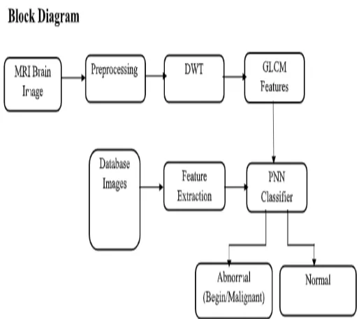
ABSTRACT: Automatic defects detection in MR images is very important in many diagnostic and therapeutic applications. Because of high quantity data in MR images and blurred boundaries, tumour segmentation and classification is very hard. This work has introduced one automatic brain tumour detection method to increase the accuracy and yield and decrease the diagnosis time. The goal is classifying the tissues to three classes of normal, begin and malignant. . In MR images, the amount of data is too much for manual interpretation and analysis. During past few years, brain tumour segmentation in magnetic resonance imaging (MRI) has become an emergent research area in the field of medical imaging system. Accurate detection of size and location of brain tumour plays a vital role in the diagnosis of tumour. The diagnosis method consists of four stages, pre-processing of MR images, feature extraction, and classification. The features selection are based on Discrete wavelet transformation (DWT).and feature extraction based GLCM . In the last stage, Probabilistic Neural Network is employed to classify the Normal and abnormal brain.

KEYWORDS: MR images, GLCM, DWT, PNN.

I. INTRODUCTION

MRI Images

Resonance Imaging- Magnetic Magnetic Resonance Image Segmentation .Segmentation of medical imagery is a challenging task due to the complexity of the images, as well as to the absence of models of the anatomy that fully capture the possible deformations in each structure. Brain tissue is a particularly complex structure, and its segmentation is an important step for derivation of computerized anatomical atlases, as well as pre- and intra-operative guidance for Therapeutic intervention. MRI segmentation has been proposed for a number of clinical investigations of varying complexity. Applications of MRI segmentation include the diagnosis of brain trauma where white matter lesions, a signature of traumatic brain injury, may potentially be identified in moderate and possibly mild cases. These

methods, in turn,

(2)

I

nternational

J

ournal of

I

nnovative

R

esearch in

S

cience,

E

ngineering and

T

echnology

II. EXISTING SYSTEMS

Threshold technique is one of the important techniques in image segmentation. This technique can be expressed as

Global Thresholding

Global (single) Thresholding method is used when there the intensity distribution between the objects of foreground and background are very distinct. When the differences between foreground and background objects are very distinct, a single value of threshold can simply be used to differentiate both objects apart. Thus, in this type of thresholding, the value of threshold T depends solely on the property of the pixel and the grey level value of the image. Some most common used global thresholding methods are Otsu method, entropy based thresholding, etc. Otsu’s algorithm is a popular global thresholding technique. Moreover, there are many popular thresholding techniques

traditional Thresholding (Otsu’s Method) In image processing, segmentation is often the first step to pre-process images to extract objects of interest for further analysis. Segmentation techniques can be generally categorized into two frameworks, edge-based and region based approaches. As a segmentation technique, Otsu’s method is widely used in pattern recognition, document binarization, and computer vision. In many cases Otsu’s method is used as a pre-processing technique to segment an image for further pre-processing such as feature analysis and quantification. Otsu’s method searches for a threshold that minimizes the intra-class variances of the segmented image and can achieve good results when the histogram of the original image has two distinct peaks, one belongs to the background, and the other belongs to the foreground or the signal. The Otsu’s threshold is found by searching across the whole range of the pixel values of the image until the intra-class variances reach their minimum. As it is defined, the threshold determined by Otsu’s method is more profoundly determined by the class that has the larger variance, be it the background or the foreground. As such, Otsu’s method may create suboptimal results when the histogram of the image has more than two peaks or if one of the classes has a large variance

Local Thresholding

(3)

I

nternational

J

ournal of

I

nnovative

R

esearch in

S

cience,

E

ngineering and

T

echnology

• Definition of edges

- Edges are significant local changes of intensity in an image.

- Edges typically occur on the boundary between two different regions in an image.

• Goal of edge detection

- Produce a line drawing of a scene from an image of that scene

. - Important features can be extracted from the edges of an image (e.g., corners, lines, curves). - These features are used by higher-level computer vision algorithms (e.g., recognition).

Canny Edge Detection

The main aims of the Canny Edge Detector are as follows: (a) Good detection - There should be a low probability of failing to mark real edge points, and low probability of falsely marking no edge points. Since both these probabilities are monotonically decreasing functions of the output signal-to-noise ratio, this criterion corresponds to maximizing signal-to-noise ratio. So basically, we need to mark as many real edges as possible. (b) Good localization - The points marked out as edge points by the operator should be as close as possible to the centre of the true edge. In essence, the marked out edges should be as close to the edges in the real edges as possible. (c) Minimal response - Only one response to a certain edge. This is implicitly captured in the first criterion since when there are two responses to the same edge, one of them must be considered false. So, the idea is that an edge should be marked only once, and image noise should not create false edges. To satisfy these requirements, John F. Canny used the calculus of variations - a technique which finds the function which optimizes a given functional. The optimal function in Canny’s detector is described by the sum of four exponential terms, but it can be approximated by the first derivative of a Gaussian. A Now, we need to convert the ideas of detection and localization into a mathematical form that is solvable. For the signal-to-noise ratio and localization, we let the impulse response of the filter to be f(x) and the edge itself to be G(x). We go on to assume that the edge is centered at x = 0. Then, the response of the filter to this edge at its center HG is given by the convolution integral

III. PROPOSED SYSTEM

(4)

I

nternational

J

ournal of

I

nnovative

R

esearch in

S

cience,

E

ngineering and

T

echnology

Dual-Tree complex Wavelet Transform:-

The dual-tree complex DWT of a signal x is implemented using two critically-sampled DWTs in parallel on the same data.

The transform is 2-times expansive because for an N-point signal it gives 2N DWT coefficients. If the filters in the upper and lower DWTs are the same, then no advantage is gained.

However, if the filters are designed is a specific way, then the sub band signals of the upper DWT can be interpreted as the real part of a complex wavelet transform, and sub band signals of the lower DWT can be interpreted as the imaginary part. Equivalently, for specially designed sets of filters, the associated with the upper DWT can be an approximate Hilbert transform of the wavelet associated with the lower DWT.

GRAY LEVEL CO-OCCURRENCE MATRIX

It is the most classical second-order statistical method for texture analysis.

An image is composed of pixels each with an intensity (a specific gray level), the GLCM is a tabulation of how often different combinations of gray levels co-occur in an image or image section. Texture feature calculations use the contents of the GLCM to give a measure of the variation in intensity at the pixel of interest. GLCM texture feature operator produces a virtual variable which represents a specified texture calculation on a single beam echogram.

Steps for virtual variable creation: Quantize the image data

Each sample on the echogram is treated as a single image pixel and its value is the intensity of that pixel. These intensities are then further quantized into a specified number of discrete gray levels, known as Quantization.

Create the GLCM

It will be a square matrix N x N in size where N is the Number of levels specified under Quantization. Steps for matrix creation are:

Let s be the sample under consideration for the calculation. Let W be the set of samples surrounding sample s which fall within a window centered upon sample s of the size specified under Window Size. Define each element i, j of the GLCM of sample present in set W, as the number of times two samples of intensities i and j occur in specified Spatial relationship. The sum of all the elements i, j of the GLCM will be the total number of times the specified spatial relationship occurs in W.Make the GLCM symmetric: Make a transposed copy of the GLCM. Add this copy to the GLCM itself.

This produces a symmetric matrix in which the relationship i to j is indistinguishable for the relationship j to i.Due to summation of all the elements i, j of the GLCM will now be twice the total number of times the specified spatial relationship occurs in W.

Normalize the GLCM:

Divide each element by the sum of all elements.

(5)

I

nternational

J

ournal of

I

nnovative

R

esearch in

S

cience,

E

ngineering and

T

echnology

Define each element i, j of the GLCM of sample present in set W, as the number of times two samples of intensities i and j occur in specified Spatial relationship. The sum of all the elements i, j of the GLCM will be the total number of times the specified spatial relationship occurs in W.

Make the GLCM symmetric:

Make a transposed copy of the GLCM. Add this copy to the GLCM itself. This produces a symmetric matrix in which the relationship i to j is indistinguishable for the relationship j to i.

Due to summation of all the elements i, j of the GLCM will now be twice the total number of times the specified spatial relationship occurs in W.

Normalize the GLCM:

Divide each element by the sum of all elements.

The elements of the GLCM may now be considered probabilities of finding the relationship i, j (or j, i) in W.

Calculate the selected Feature. This calculation uses only the values in the GLCM. For e.g.Energy, Entropy, Contrast,

Homogeneity, Correlation.

The sample s in the resulting virtual variable is replaced by the value of this calculated feature.

Calculate the selected Feature. This calculation uses only the values in the GLCM.

The sample s in the resulting virtual variable is replaced by the value of this calculated feature.

GLCM directions of Analysis

• Horizontal (0⁰)

• Vertical (90⁰)

• Diagonal:

• Bottom left to top right (-45⁰)

• Top left to bottom right (-135⁰)

Denoted P₀, P₄₅, P₉₀, & P₁₃₅ Respectively. Ex. P₀ (i, j)

GLCM of an image is computed using a displacement vector d, defined by its radius δ and orientation θ.

(6)

I

nternational

J

ournal of

I

nnovative

R

esearch in

S

cience,

E

ngineering and

T

echnology

ENERGY

Also called Uniformity or Angular second moment. Measures the textural uniformity that is pixel pair repetitions. Detects disorders in textures. Energy reaches a maximum value equal to one.

ENTROPY

Measure the disorder of complexity of an image

The entropy is large when the image is not texturality .uniform Entropy is strongly but inversely corrected to energy

p(x,y) is the GLC M

CONTRAST

Measure the spatial frequency of an image and it difference moment of GLCM

It is the difference between the highest and the lowest valves of a contiguous set of pixels It is measures the amount of local variations present in the image

HOMOGENEITY

Also it is called inverse difference moment

Measures the image homogeneity as it assumes larger values for smaller gray tones differences in pair elements. It is more sensitive to the presence of near diagonal element in the GLCM

It has maximum value when all elements in the image are same. Homogeneity decrease If contrast increase while energy kept constant.

Homogeneity=sum(sum(p(x,y)/(1 + [x-y])))

Probabilistic neural network (PNN)

A probabilistic neural network (PNN) is a feed forward neural network which is widely used in classification and pattern recognition problems. In the PNN algorithm, the parent probability distribution function (PDF) of each class is approximated by a Parson window and a non-parametric function. Then, using PDF of each class, the class probability of a new input data is estimated and Bayes’ rule is then employed to allocate the class with highest posterior probability to new input data. By this method, the probability of mi-classification is minimized.. In a PNN, the operations are organized into a multilayered feed forward network with four layers:

• Input layer

• Hidden layer

• Pattern layer/Summation layer

• Output layer

• Diagram

(7)

I

nternational

J

ournal of

I

nnovative

R

esearch in

S

cience,

E

ngineering and

T

echnology

Input layer

Each neuron in the input layer represents a predictor variable. In categorical variables, N-1 neurons are used when there are N number of categories. It standardizes the range of the values by subtracting the median and dividing by the interquartile range Then the input neurons feed the values to each of the neurons in the hidden layer.

Hidden layer

This layer contains one neuron for each case in the training data set. It stores the values of the predictor variables for the case along with the target value. A hidden neuron computes the Euclidean distance of the test case from the neuron’s center point and then applies the kernel function using the sigma values.

Summation layer

For PNN networks there is one pattern neuron for each category of the target variable. The actual target category of each training case is stored with each hidden neuron; the weighted value coming out of a hidden neuron is fed only to the pattern neuron that corresponds to the hidden neuron’s category. The pattern neurons add the values for the class they represent.

Output layer

output layer

(8)

I

nternational

J

ournal of

I

nnovative

R

esearch in

S

cience,

E

ngineering and

T

echnology

Diagram

Advantages

• PNNs are much faster than multilayer perception networks. • PNNs can be more accurate than multilayer perception networks. • PNN networks are relatively insensitive to outliers.

• PNN networks generate accurate predicted target probability scores. • PNNs approach Bayes optimal classification

SOFTWARE REQUIREMENTS: Python:

• Python is an interpreted, high-level, general-purpose programming language. • It provides constructs that enable clear programming on both small and large scales. • Python features a dynamic type system and automatic memory management .

• It supports multiple programming paradigms, including object- oriented, imperative, functional and procedural , and has a large and comprehensive standard library.

• Python interpreters are available for many operating systems.

• CPython, the reference implementation of python, is open source software and has a community-based development model, as do nearly all of python’s other implementations.

• Python and cpython are managed by the non-profit python software foundation.

IV. CONCLUSION

(9)

I

nternational

J

ournal of

I

nnovative

R

esearch in

S

cience,

E

ngineering and

T

echnology

wavelet transformation (DTCWT). In the last stage, Probabilistic Neural Network is employed to classify the Normal and abnormal brain.

REFERENCES

[1] R. J. Gillies, P. E. Kinahan, and H. Hricak, “Radiomics: Images are more than pictures, they are data,” Radiology, vol. 278, no. 2, pp. 565–580, 2015.

[2] H. J. Aerts et al., “Decoding tumour phenotype by noninvasive imaging using a quantitative radiomics approach,” Nature Commun., vol. 5, Jun. 2014, Art. no. 4006.

[3] T. P. Coroller et al., “CT-based radiomic signature predicts distant metastasis in lung adenocarcinoma,” Radiotherapy Oncol., vol. 114, no. 3, pp. 345–350, 2015

[4] C. Parmar et al., “Radiomic feature clusters and prognostic signatures specific for lung and head & neck cancer,” Sci. Rep., vol. 5, Jun. 2015, Art. no. 11044.