Electronic Thesis and Dissertation Repository
8-15-2016 12:00 AM
Modeling the Mass Function of Stellar Clusters Using the
Modeling the Mass Function of Stellar Clusters Using the
Modified Lognormal Power-Law Probability Distribution Function
Modified Lognormal Power-Law Probability Distribution Function
Deepakshi Madaan
The University of Western Ontario
Supervisor
Dr. Shantanu Basu
The University of Western Ontario
Graduate Program in Applied Mathematics
A thesis submitted in partial fulfillment of the requirements for the degree in Master of Science © Deepakshi Madaan 2016
Follow this and additional works at: https://ir.lib.uwo.ca/etd
Part of the Applied Mathematics Commons, and the Stars, Interstellar Medium and the Galaxy Commons
Recommended Citation Recommended Citation
Madaan, Deepakshi, "Modeling the Mass Function of Stellar Clusters Using the Modified Lognormal Power-Law Probability Distribution Function" (2016). Electronic Thesis and Dissertation Repository. 4045.
https://ir.lib.uwo.ca/etd/4045
This Dissertation/Thesis is brought to you for free and open access by Scholarship@Western. It has been accepted for inclusion in Electronic Thesis and Dissertation Repository by an authorized administrator of
Abstract
We use the Modified Lognormal Power-law (MLP) probability distribution function to model the behaviour of the mass function (MF) of young and populous stellar populations in di↵erent environments. We begin by modeling the MF of NGC1711, a simple stellar
pop-ulation (SSP) in the Large Magellanic Cloud as a pilot case. We then use model selection criterion to rank di↵erent candidate models. Using the MLP we find that the stellar catalogue
of NGC1711 follows a pure power-law behaviour below the completeness limit with the slope
↵ = 2.75 for dN/dlnm / m ↵+1 in the mass range 0.89 M to 7.75 M . Furthermore, we explore that the MLP takes a truncated form for fixed stopping time for accretion. By using model selection criterion, we conclude that the MLP serves as the most useful candidate to model lognormal, power-law or hybrid behaviour of the MF.
Keywords: stellar clusters, star formation, luminosity function, mass function, data analy-sis, Magellanic Clouds, model selection, regression
This thesis has been written by Deepakshi Madaan under the supervision of Dr. Shantanu Basu. The work in chapter two is also in collaboration with Sophia Lianou and is nearing submission to Monthly Notices of the Royal Astronomical Society. The work in chapter three is in prepa-ration for submission.
Acknowlegements
First and foremost, I am extremely thankful to my supervisor Dr. Shantanu Basu for his im-mense support and his belief in my ability when I felt otherwise sometimes. I not only have learnt so much under his guidance, but have had as much fun learning as possible. His words and motivation, I know would help me go a long way. I am really thankful to him for also mak-ing all of us, the research group, feel like at home with the many get togethers and trips. I am also very thankful to Sophia Lianou, for having found not just a mentor/collaborator but also a
friend in her. She is an inspiring woman who helps me do my work with more dedication and enthusiasm. Not to forget my research mates: Sayantan, Pranav, Mark, and Andy who have made this process so much easier and help me find a home away from home. Most importantly, I couldn’t have achieved any of this without the unconditional support of my family and the two friends: Alina and Nashi who have been through thin and thick with me. I would also like to extent my heartiest thanks to Audrey, Cinthia, Brian and Dr. Wahl for helping me in the transition and answering my never-ending inquiries. Dr. Corless, Dr. Barmby, Dr. Sigut, Dr. Houde, and Dr. Reid, all have helped me to engage in rigorous learning and critical thinking and I am really thankful for that. Lastly, I just want to say: Mom, Dad, didi and bhai, I hope I made you proud.
Abstract ii
Co-Authorship Statement ii
Acknowlegements iv
List of Figures vii
List of Tables viii
List of Appendices ix
1 Introduction 1
1.1 Mass Function . . . 2
1.1.1 From Luminosity to Mass . . . 3
1.2 IMF Models . . . 3
1.3 Modified Lognormal Power-Law Probability Distribution Function . . . 5
1.3.1 Physical Motivation and Derivation . . . 6
1.3.2 PDF and Properties . . . 7
1.4 Young stellar populations . . . 8
1.5 Model Fitting and Model Selection . . . 9
1.5.1 Non-Linear Regression . . . 9
1.5.2 Maximum Likelihood Estimation . . . 10
1.6 Thesis Statement and Contribution . . . 11
Bibliography . . . 11
2 Modeling the Mass Function of NGC 1711 as a Case Study using the MLP 19 2.1 From Luminosity to Mass . . . 19
2.1.1 Luminosity Function . . . 20
2.1.2 Mass Luminosity Relation . . . 22
2.2 Mass Function . . . 23
2.3 MLP modeling of the Mass Function . . . 25
2.3.1 Fitting Results . . . 25
2.3.2 Truncated MLP . . . 29
2.3.3 MLP as a hybrid . . . 30
2.4 Summary . . . 32
Bibliography . . . 33
3 Model Selection: Which Model to choose for the IMF of Young Stellar Clusters? 36 3.1 Observational data . . . 37
3.2 IMF Models and Parameter Estimation . . . 37
3.3 Model Selection using Information Criterion . . . 43
3.4 Discussion . . . 45
Bibliography . . . 46
4 Conclusion 49 Bibliography . . . 50
A Derivation of the MLP 52
B Joint Likelihood Function 53
Curriculum Vitae 54
2.1 Color Magnitude Diagram . . . 20
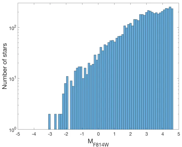
2.2 Apparent Magnitude Histogram . . . 21
2.3 Luminosity Function Histogram . . . 22
2.4 Isochrones Plot . . . 23
2.5 Mass-Magnitude Relation Plot . . . 24
2.6 Mass Function Histogram . . . 24
2.7 Log Mass Function Plot . . . 25
2.8 MLP fit for Padova isochrone . . . 26
2.9 MLP fit for MESA isochrone . . . 26
2.10 Residuals Plot . . . 28
2.11 QQ Plot . . . 28
2.12 Truncated MLP . . . 29
2.13 MLP Hybrid Plot . . . 31
3.1 ONC plot . . . 41
3.2 NGC 1711 plot . . . 41
3.3 NGC 6611 plot . . . 42
3.4 NGC 2024 plot . . . 42
List of Tables
3.1 Chabrier IMF best fit parameters table . . . 40
3.2 Kroupa IMF best fit parameters table . . . 40
3.3 MLP best fit parameters table . . . 40
3.4 ONC likelihood table . . . 44
3.5 NGC 1711 likelihood table . . . 44
3.6 NGC 6611 likelihood table . . . 44
3.7 NGC 2024 likelihood table . . . 45
Appendix A Derivation of the MLP . . . 52 Appendix B Joint Likelihood Function . . . 53
Chapter 1
Introduction
For any star with a given chemical composition, its mass determines its structure and evolution by the Vogt-Russell theorem [5]. Once the mass of the star is known, we can find various stellar properties such as luminosity, radius, and radiation spectrum. Also, various integrated properties of any group of stars, i.e. a star cluster or a galaxy, depend on how stellar masses are distributed into di↵erent mass intervals [54]. Hence, it is necessary to study the distribution of
stellar masses at birth, known as the initial mass function (IMF), in di↵erent environments to
understand stellar population evolution and further galaxy evolution.
The question of universality of the IMF in di↵erent environments, i.e. whether the shape
of the IMF is universal for stellar populations formed under di↵erent cloud conditions, is one
of the most fundamental questions in astrophysics today [46]. There are various schools of thought that favor universality [5, 33] while many others argue otherwise [18, 41]. Dib, in 2014, does a thorough investigation of the universality of the IMF using Bayesian statistics with a sample of eight young stellar clusters. He concludes that the shape of the IMF does depend on the environment of star formation [18]. Even though various studies have been done using Bayesian statistics to study universality of the IMF, the problem of model fitting and model selection (i.e. which model best represents the underlying population) has rarely been comprehensively addressed. Model selection is used to study and compare di↵erent
ical models [40, 39, 57, 60], but no such study for model selection of IMF models has yet been done.
1.1 Mass Function
The distribution of stellar masses at birth in a star forming event into di↵erent mass intervals is
called the initial mass function (IMF). The process of star formation is a highly complex and difficult-to-predict transformation of molecular clouds in the interstellar medium, controlled by
various physical mechanisms such as self-gravity, turbulence, and magnetic fields [32, 46, 8, 44]. Thus, the process of star formation can be considered as a stochastic process and the mass of a star a continuous random variable [54]. Therefore, we can model the fraction of stars in each mass interval i.e the mass function (MF) as a probability density function (pdf).
If mass m of a star is considered as a continous random variable which is distributed ac-cording to a pdf f(m), assuming the pdf is independent of space and time, then f(m)dmgives the number of stars in some volume of space in the interval [m,m+dm] [53, 54, 13],
f(m)= d(N/V)
dm , (1.1)
whereN=Number of stars in the interval [m,m+dm] ,V =Volume.
The usual practice is to divide the intervals into log masses i.e. take the pdf as f(log m) which is called the MF i.e. the mass function,
f(log m)= d(N/V)
dlog m , (1.2)
f(log m)= d(N/V)
dm
dm
dlog m, (1.3)
f(log m)= (ln10)m f(m), (1.4)
For simplicity, we take the MF as f(ln m) for our study i.e. f(ln m) = m f(m). f(log m) gives
1.2. IMF Models 3
1.1.1 From Luminosity to Mass
The main source of direct and accurate measurement of the dynamical mass of any star is studying a binary system [2, 59]. The data on stellar masses are usually acquired from eclips-ing binaries whereby useclips-ing light curves and radial velocity measurements along with Kepler’s laws one can accurately determine the masses of individual stars [21, 61]. For stars that are not formed in binaries, masses are obtained from a luminosity to mass conversion. Mass is ob-tained from luminosity using theoretical stellar evolutionary models that give mass-luminosity relations (MLR) or mass-magnitude1 relations (MMR) [52, 55, 56, 27, 26, 25]. Once these models are computed, they are checked against the observed dynamical mass in binaries for authenticity. A number of such evolutionary2/isochrone models3 have been derived over the years such as Barra↵e [4], D’Antona & Mazzitelli [17], Padova [9], Geneva [36], MESA [51].
All these models di↵er in various physical inputs and initial conditions.
The masses of stars are derived from their luminosities using two di↵erent set of
evolution-ary models in Chapter 2. In Chapter 3, the data obtained for stellar masses are obtained directly from literature where various authors use di↵erent evolutionary models to obtain the MF.
1.2 IMF Models
The choice of the functional form of the pdf is significant since it is used as an important tool for various calculations in stellar population synthesis [10]. Predictions of luminosity functions of white dwarfs depend on the IMF [16]. We can also study the rate of formation of planetary nebulae using the IMF [50]. The IMF enters into the equations to study chemical evolution of galaxies [58]. Since many astrophysical studies depend on the functional form of the IMF, it is important to choose a simple analytical and integrable form of the pdf that
1The brightness of a star measured on a logarithmic scale is the apparent magnitude of a star.
2Evolutionary models are plotting of evolutionary tracks of stars of di↵erent masses on the
Hertzsprung-Russell Diagram (H-R Diagram). H-R Diagram is a plot of e↵ective temperature/spectral class vs.
luminos-ity/absolute magnitude of a star.
adequately represents the mass distribution. Not only that but more importantly the choice of the functional form should underlie a physical motivation that bears origin from a theory of star formation, even though the process of star formation is yet to be fully understood.
In 1955, Salpeter was the first to provide the stellar initial mass distribution with an analytic power law pdf approximation : dN/dm / m ↵ with↵= 2.35 ordN/dln m / m 1.35 [53]. He did so by studying the Luminosity function (LF) of main sequence stars of over the mass range 0.4M <m<10M in the solar neighbourhood.
Subsequently, Miller and Scalo suggested a lognormal form for masses 0.1M < m <
50M on finding that the stellar mass distribution flattens for low mass stars [42]. Later in 1984, Zinnecker gave a theoretical explanation to Miller and Scalo’s lognormal form of the IMF by invoking the Central Limit Theorem (CLT) [62]. According to the CLT, the sum of a large number of independent and identically distributed random variables will follow a Gaus-sian distribution [1]. Since the process of star formation is a highly complex transformation controlled by various physical processes, the formation of stellar mass can be considered as a product of a large number of independent and identically distributed random variables deter-mined by the processes. Thus by the CLT the log of the product of the random variables will follow a Gaussian distribution, implying the stellar mass follows a lognormal pdf [62].
Chabrier proposed a lognormal form for the substellar and low mass stellar regime i.e. m<
1M along with a power-law representation for intermediate and high mass stellar regime [14, 13],
f(log m)/
8 >>>>> < >>>>> : 1 p
2⇡ exp
" (log m log m
c)2
2 2
#
m 1M
m ↵+1 m> 1M
(1.5)
where ↵ > 1. The paramteer mc corresponds to the characteristic mass that the lognormal
takes which also is the mean of the distribution while represents the spread of the lognormal distribution and↵is the slope of the power-law.
1.3. ModifiedLognormalPower-LawProbabilityDistributionFunction 5
regimes [35, 34, 33].
f(m)/m ↵ : 8 >>>>> >>>< >>>>> >>>:
↵= +0.3±0.7 0.01M m< 0.08M ↵= +1.3±0.5 0.08M m< 0.50M
↵= +2.3±0.3 0.50M m
(1.6)
The functional forms Salpeter, Chabrier and Kroupa are the most widely used functional forms for the MF with total number of parameters as 2, 4, and 4, respectively. With models like the Chabrier and Kroupa having to do with joining conditions or the lack of physical motiva-tion, the need of a model to represent the MF of stellar populations as a single function with a simple analytical and integrable form bearing a physical motivation is noteworthy. Hence, the Modified Lognormal Power-law Probability (MLP) distribution function proposed by Basu & Jones in 2004 can be looked at as a good analytical approximation for the mass distribution of stellar populations [6].
1.3 Modified Lognormal Power-Law Probability
Distribu-tion FuncDistribu-tion
lognormal-like and power law-like behaviour.
1.3.1 Physical Motivation and Derivation
Basu & Jones [7] used a statistical approach to model the subsequent growth of masses by accretion in the process of star formation, which results in a power-law distribution starting from an initial lognormal distribution.
Since the formation of a star is the result of various physical mechanisms, the mass of a star can be written asm= f1⇥ f2⇥...⇥ fN. Thus according to the CLT, for largeN, lnmfollows
a Gaussian distribution [62] i.e.mfollows a lognormal distribution with meanµ0and standard deviation 0. Starting from an initial lognormal form, Basu and Jones explored the idea of the growth of the mass of a star due to accretion [7]:
dm
dt = m,m(t)=m0exp( t), (1.7)
m0is the initial mass that follows a lognormal distribution and is the growth rate. The mean
of the distribution becomes µ = µ0 + t while the standard deviation remains 0. Assuming an exponential distribution for accretion time i.e. f(t) = e t where is the death rate for
accretion, the pdf for stellar mass becomes4:
Z 1
0
1 p
2⇡ 0m
exp (ln m µ0 t)2
2 02 e
tdt
= ↵0
2 exp
⇣
↵0µ0+↵20 20/2
⌘
m (1+↵0)⇥
erfc p1
2 ↵0 0
lnm µ0 0
!! !
(1.8)
where↵0 = / .The exponential growth of masses due to accretion gives a power-law tail to the underlying lognormal distribution of initial masses.
1.3. ModifiedLognormalPower-LawProbabilityDistributionFunction 7
1.3.2 PDF and Properties
The MLP function is a three-parameter pdf. The three parameters of the distribution function are ↵0, µ0, and 0. ↵0 + 1 is the power-law index of dNdm for the power-law distribution: characteristic of a Pareto distribution which is used to represent pure power-law distributions. The parametersµ0 and 20 are the same as for the lognormal distribution but do not represent the mean and variance of the distribution unlike for the lognormal distribution. Parametersµ0 and 0describe the shape of the lognormal-like body and↵0 represents the power-law tail. In the limit as 0 tends to zero, the function behaves as a pure power-law.
If mis the the mass of a star, the pdf of the MLP function is given in the closed form as [6]:
f(m)= ↵0
2 exp
⇣
↵0µ0+↵20 20/2
⌘
m (1+↵0)⇥erfc p1
2 ↵0 0
lnm µ0 0
!!
, m2[0,1),
Some properties of the MLP function are: (i) Raw Moments:
E[Mk]= ↵0
↵0 kexp 2 0k2 2 +µ0k
!
, ↵0> k. (1.9)
(ii) Variance:
Var(M)= E[M2] (E[M])2 =↵0exp( 20+2µ0)
0 BBBB@ e 20
↵0 2
↵0 (↵0 1)2
1
CCCCA, ↵0 > 2.
(iii) Cumulative Distribution Function:
FM(m;↵0, µ0, 0)= 1 2erfc
ln(m) µ0 p
2 0
! 1
2exp ↵0µ0+ ↵20 20
2
!
m ↵0erfc ↵p0 0
2
ln(m) µ0 p
2 0
!
.
(1.10) (iv) Mode: Solving the following transcendental equation will give us the mode of the distri-bution
f0(m)= 0 () Kerfc(u)=e u2
where
K = 0(↵0+1)
r ⇡ 2,u=
1 p
2 ↵0 0
lnm µ0 0
!
. (1.12)
1.4 Young stellar populations
We have initiated a study to apply the MLP function for the investigation of the IMF in young and populous star clusters. Star clusters are considered as simple stellar populations with the same chemical composition and age [45], making them ideal targets for IMF studies.
In chapter 2, we present a pilot study introducing our method and its application to NGC 1711, a young and populous star cluster in the Large Magellanic Cloud (LMC). LMC is a gas-rich satellite galaxy of the Milky Way located at a distance of ⇠50 kpc [23]. Overall, the star clusters in the LMC span a wide range in ages (106 yr to 1010 yr) and masses (10 to 106 M ) [28]. NGC 1711 is located in the north-west part of the LMC, below its bar. NGC 1711 is a populous young star cluster, with an age of 107.7±0.05 in logarithmic space, a metallicity5 of -0.57±0.17 dex and and a reddening6E(B-V) of 0.09±0.03 [19].
In chapter 3, we take masses for three young and populous clusters: Orion Nebula Cluster (ONC), NGC 2024, and NGC6611 from the literature directly. These three clusters were taken because they vary in their mass ranges and their MFs show di↵erent behaviour. ONC is the
nearest cluster with plenty of massive O and B stars located at a distance of 400 pc from the sun. Various groups like Hillenbrand [24], Palla and Stahler [49], Andersen [3] have studied the stellar content of the ONC. We consider the census reviewed by Hillenbrand [24] and Da Rio et al. [15] to get a complete sample of mass range between 0.029 M and 45.7 M . Both Hil-lenbrand and Da Rio et al. derived the masses using D’Antona & Mazzitelli [17]evolutionary tracks. NGC2024 is a young cluster rich in brown dwarfs and low mass stars. Levine et al. [38] conducted a near-infrared spectroscopic study of this young cluster and obtained a mass range
5Elements other than hydrogen and helium are called as metals in astrophysics. Metallicity is the ratio of metal
content to hydrogen and helium content.
6Interstellar reddening is a phenomena where stars appear more red in color due to absorption or scattering of
1.5. ModelFitting andModelSelection 9
of 0.02 M and 0.72 M using the Bara↵e et al. [4] evolutionary tracks. NGC6611 is also a
young cluster useful to study the low mass IMF but also helps in probing higher i.e. interme-diate stellar masses. Using the Bara↵e et al. [4] evolutionary models, Oliveira et al. [48, 47]
obtain a mass range of 0.01M to 6.04M for the age of the cluster as 2 million years.
1.5 Model Fitting and Model Selection
Given a sample of observations and a set of candidate mathematical models to describe the data set, the problem of model fitting and model selection comes into play. For model fitting one first needs to investigate whether a mathematical model can be considered as a candidate model or not which can be done using non-linear regression for a non-linear model. Regression finds best fit parameter values for the model by minimizing the sum of the squared errors. A more robust way of parameter estimation is by using maximum likelihood estimation that also aims at minimizing the residuals between the mathematical model and the underlying data set. Once the set of candidate models have been established, model selection helps in finding the best candidate model [11].
1.5.1 Non-Linear Regression
Regression is a statistical technique that analyzes the relationship between a dependent variable and several independent variables [22]. It is the process of fitting a mathematical equation of several unknown parameters to the experimental data presuming that the equation is a correct mathematical description of the underlying process [29]. The main objective of a non-linear least squares method is to estimate the unknown parameters of the mathematical equation by minimizing the sum of squares of the residual [43]. We use the Levenberg Marquardt method on the normalized MF to estimate the best-fit parameters for the MLP function.
methods to compute the estimates for the parameters of the given equation with maximum like-lihood whilst ignoring the limitations of both these methods. The method of Steepest Descent is advantageous in initial iterations as it quickly moves along the direction of steepest descent to minimize the sum of squares of the residuals, but becomes less accurate on later iterations. Unlike the Steepest Descent method, Gauss Newton method is e↵ective for later iterations but
may go in the wrong direction for initial iterations. Hence, the LM method jumps from the Steepest Descent to the Gauss Newton method from initial to later iterations [37]. Likewise the Method of Steepest Descent and Gauss Newton Method, the LM method is an iterative process and requires an initial estimation of the parameters. It tries to find a better estimate to the parameters by minimizing the sum of the squares of the residuals. To check whether the algorithm gives us the best fitting parameters, an understanding of how good the fit is and the uncertainty involved is fundamental.
1.5.2 Maximum Likelihood Estimation
Given a sample of observations x1, x2, x3, ..., xn where xi0s are independent and identically
distributed data points assumed to be taken from a pdf f(X|⇥) of k unknown parameters
✓1, ✓2, ..., ✓k, the likelihood function can be defined as [30]:
L(⇥|xi)= f(x1|⇥)f(x2|⇥)...f(xn|⇥)= n
Y
i=1
f(xi|⇥), (1.13)
Note thatL(⇥|xi) is a function of the unknown parameters with data points kept fixed unlike the
pdf which is a function of observations with fixed parameter values. Maximizing the likelihood function helps in finding the parameter values that are most likely to describe the data set. For simplicity the log of the likelihood function is maximized i.e.:
ln L(⇥|xi)= ln f(x1|⇥)+ ln f(x2|⇥)+ ...+ ln f(xn|⇥)= n
X
i=1
ln f(xi|⇥), (1.14)
simulta-1.6. ThesisStatement andContribution 11
neously solving for:
d ln L(⇥|xi)
d✓j = 0 : j=1, ....,k. (1.15)
For various distributions like the lognormal distribution or the Pareto distribution, functional forms can be found for the maximum likelihood estimators but for distributions that do not have an analytic form for the estimators, global optimization techniques such as simulated annealing or particle swarm are explored to find global minima for the negative-likelihood function i.e.
ln L(⇥|xi) which is same as finding global maxima for the likelihood function.
Both simulated annealing and particle swarm can be used to solve non-linear bounded opti-mization problems. Simulated annealing is an adaption of the Monte Carlo method that com-pares the objective function evaluated at a random initial number with the objective function evaluated at a neighbouring random number until it reaches the maximum number of iterations or a tolerance condition [31]. Particle Swarm on the other hand is also an iterative method that moves around in search space according to some mathematical formulae to find the optimal solution to the problem [20].
1.6 Thesis Statement and Contribution
Our goal in Chapter 2 is to determine whether the distribution of stars in NGC 1711 can best be described by a power law, a lognormal or a hybrid function. As NGC 1711 is a young and populous star cluster, this provides us with a statistically significant sample of stars, ranging over a wide mass domain to be able to model the high mass stellar regime. In Chapter 3, we model the MF of di↵erent young and populous star clusters from the literature in various
environments using di↵erent functions. We then use a model selection criterion to determine
[1] John Aitchison and James A C Brown. The lognormal distribution with special reference to its uses in economics. Cambridge Univ. Press, London, 1957.
[2] Johannes Andersen. Accurate masses and radii of normal stars. The Astronomy and Astrophysics Review, 3(2):91–126, 1991.
[3] M. Andersen, M. R. Meyer, M. Robberto, L. E. Bergeron, and N. Reid. The low-mass initial mass function in the Orion nebula cluster based on HST/NICMOS III imaging.
A&A, 534:A10, October 2011.
[4] I. Bara↵e, G. Chabrier, F. Allard, and P. H. Hauschildt. Evolutionary models for solar
metallicity low-mass stars: mass-magnitude relationships and color-magnitude diagrams.
A&A, 337:403–412, September 1998.
[5] N. Bastian, K. R. Covey, and M. R. Meyer. A Universal Stellar Initial Mass Function? A Critical Look at Variations. ARA&A, 48:339–389, September 2010.
[6] S. Basu, M. Gil, and S. Auddy. The MLP distribution: a modified lognormal power-law model for the stellar initial mass function. MNRAS, 449:2413–2420, May 2015.
[7] S. Basu and C. E. Jones. On the power-law tail in the mass function of protostellar condensations and stars. MNRAS, 347:L47–L51, January 2004.
[8] I. A. Bonnell, R. B. Larson, and H. Zinnecker. The Origin of the Initial Mass Function.
Protostars and Planets V, pages 149–164, 2007.
BIBLIOGRAPHY 13
[9] A. Bressan, P. Marigo, L. Girardi, B. Salasnich, C. Dal Cero, S. Rubele, and A. Nanni. PARSEC: stellar tracks and isochrones with the PAdova and TRieste Stellar Evolution Code. MNRAS, 427:127–145, November 2012.
[10] G. Bruzual and S. Charlot. Stellar population synthesis at the resolution of 2003.MNRAS, 344:1000–1028, October 2003.
[11] Kenneth P Burnham and David R Anderson. Multimodel inference understanding aic and bic in model selection. Sociological methods&research, 33(2):261–304, 2004.
[12] Bradley W Carroll and Dale A Ostlie. An introduction to modern astrophysics and cos-mology, volume 1. 2006.
[13] G. Chabrier. Galactic Stellar and Substellar Initial Mass Function. PASP, 115:763–795, July 2003.
[14] G. Chabrier. The Initial Mass Function: from Salpeter 1955 to 2005. In E. Corbelli, F. Palla, and H. Zinnecker, editors, The Initial Mass Function 50 Years Later, volume 327 ofAstrophysics and Space Science Library, page 41, January 2005.
[15] N. Da Rio, M. Robberto, L. A. Hillenbrand, T. Henning, and K. G. Stassun. The Initial Mass Function of the Orion Nebula Cluster across the H-burning Limit. ApJ, 748:14, March 2012.
[16] F. D’antona and I. Mazzitelli. The progenitor masses and the luminosity function of white dwarfs. A&A, 66:453–461, June 1978.
[17] F. D’Antona and I. Mazzitelli. New pre-main-sequence tracks for M less than or equal to 2.5 solar mass as tests of opacities and convection model. ApJS, 90:467–500, January 1994.
[18] S. Dib. Testing the universality of the IMF with Bayesian statistics: young clusters.
[19] B. Dirsch, T. Richtler, W. P. Gieren, and M. Hilker. Age and metallicity for six LMC clusters and their surrounding field population. A&A, 360:133–160, August 2000.
[20] Russ C Eberhart, James Kennedy, et al. A new optimizer using particle swarm theory. In
Proceedings of the sixth international symposium on micro machine and human science,
volume 1, pages 39–43. New York, NY, 1995.
[21] Z. Eker, F. Soydugan, E. Soydugan, S. Bilir, E. Yaz G¨okc¸e, I. Steer, M. T¨uys¨uz, T. S¸eny¨uz, and O. Demircan. Main-Sequence E↵ective Temperatures from a Revised
Mass-Luminosity Relation Based on Accurate Properties. AJ, 149:131, April 2015.
[22] E. D. Feigelson and G. J. Babu. Modern Statistical Methods for Astronomy. July 2012.
[23] W. L. Freedman, B. F. Madore, B. K. Gibson, L. Ferrarese, D. D. Kelson, S. Sakai, J. R. Mould, R. C. Kennicutt, Jr., H. C. Ford, J. A. Graham, J. P. Huchra, S. M. G. Hughes, G. D. Illingworth, L. M. Macri, and P. B. Stetson. Final Results from the Hubble Space Telescope Key Project to Measure the Hubble Constant. ApJ, 553:47–72, May 2001.
[24] L. A. Hillenbrand. On the Stellar Population and Star-Forming History of the Orion Nebula Cluster. AJ, 113:1733–1768, May 1997.
[25] J. Holtzman, WFPC Id Team, and WFPC2 Id Team. The Luminosity Function and Ini-tial Mass Function in the Galactic Bulge. In American Astronomical Society Meeting Abstracts, volume 29 of Bulletin of the American Astronomical Society, page 1383,
De-cember 1997.
[26] J. A. Holtzman, J. R. Mould, J. S. Gallagher, III, A. M. Watson, C. J. Grillmair, G. E. Ballester, C. J. Burrows, J. T. Clarke, D. Crisp, R. W. Evans, R. E. Griffiths, J. J. Hester,
BIBLIOGRAPHY 15
[27] D. A. Hunter. The Stellar Population and Star Clusters in the Unusual Local Group Galaxy IC 10. ApJ, 559:225–242, September 2001.
[28] D. A. Hunter, B. G. Elmegreen, T. J. Dupuy, and M. Mortonson. Cluster Mass Functions in the Large and Small Magellanic Clouds: Fading and Size-of-Sample E↵ects. AJ,
126:1836–1848, October 2003.
[29] Michael L Johnson. Why, when, and how biochemists should use least squares.Analytical biochemistry, 206(2):215–225, 1992.
[30] Norman L Johnson, Samuel Kotz, and N Balakrishnan. Continuous multivariate distri-butions, volume 1, models and applications, volume 59. New York: John Wiley & Sons,
2002.
[31] Scott Kirkpatrick, C Daniel Gelatt, Mario P Vecchi, et al. Optimization by simmulated annealing. science, 220(4598):671–680, 1983.
[32] R. S. Klessen, M. R. Krumholz, and F. Heitsch. Numerical Star-Formation Studies - A Status Report. Advanced Science Letters, 4:258–285, February 2011.
[33] P. Kroupa. On the variation of the initial mass function. MNRAS, 322:231–246, April 2001.
[34] P. Kroupa. The Initial Mass Function of Stars: Evidence for Uniformity in Variable Systems. Science, 295:82–91, January 2002.
[35] P. Kroupa, C. A. Tout, and G. Gilmore. The distribution of low-mass stars in the Galactic disc. MNRAS, 262:545–587, June 1993.
[36] T. Lejeune and D. Schaerer. Database of Geneva stellar evolution tracks and isochrones for (UBV)J(RI)C JHKLL’M, HST-WFPC2, Geneva and Washington photometric
[37] Kenneth Levenberg. A method for the solution of certain non–linear problems in least squares. Quaterly of Applied Mathematics, 2:164–168, 1944.
[38] J. L. Levine, A. Steinhauer, R. J. Elston, and E. A. Lada. Low-Mass Stars and Brown Dwarfs in NGC 2024: Constraints on the Substellar Mass Function.ApJ, 646:1215–1229, August 2006.
[39] A. R. Liddle. How many cosmological parameters? MNRAS, 351:L49–L53, July 2004.
[40] A. R. Liddle. Information criteria for astrophysical model selection. MNRAS, 377:L74– L78, May 2007.
[41] G. R. Meurer, O. I. Wong, J. H. Kim, D. J. Hanish, SUNGG, and SINGG. Evidence for a Non-Uniform Initial Mass Function in the Local Universe. InAmerican Astronomical Society Meeting Abstracts #213, volume 41 of Bulletin of the American Astronomical
Society, page 324, January 2009.
[42] G. E. Miller and J. M. Scalo. The initial mass function and stellar birthrate in the solar neighborhood. ApJ, 41:513–547, November 1979.
[43] Harvey J Motulsky and Lennart A Ransnas. Fitting curves to data using nonlinear re-gression: a practical and nonmathematical review. The FASEB journal, 1(5):365–374, 1987.
[44] T. C. Mouschovias and G. E. Ciolek. Magnetic Fields and Star Formation: A Theory Reaching Adulthood. In C. J. Lada and N. D. Kylafis, editors,NATO Advanced Science Institutes (ASI) Series C, volume 540 ofNATO Advanced Science Institutes (ASI) Series
C, page 305, 1999.
BIBLIOGRAPHY 17
[46] S. S. R. O↵ner, P. C. Clark, P. Hennebelle, N. Bastian, M. R. Bate, P. F. Hopkins,
E. Moraux, and A. P. Whitworth. The Origin and Universality of the Stellar Initial Mass Function. Protostars and Planets VI, pages 53–75, 2014.
[47] J. M. Oliveira, R. D. Je↵ries, and J. T. van Loon. The low-mass initial mass function in
the young cluster NGC6611. , 392:1034–1050, January 2009.
[48] J. M. Oliveira, R. D. Je↵ries, J. T. van Loon, S. P. Littlefair, and T. Naylor. Circumstellar
discs around solar mass stars in NGC 6611. , 358:L21–L24, March 2005.
[49] F. Palla and S. W. Stahler. Star Formation in the Orion Nebula Cluster.ApJ, 525:772–783, November 1999.
[50] K. A. Papp, C. R. Purton, and S. Kwok. The e↵ects of mass and metallicity upon planetary
nebula formation. ApJ, 268:145–154, May 1983.
[51] B. Paxton, M. Cantiello, P. Arras, L. Bildsten, E. F. Brown, A. Dotter, C. Mankovich, M. H. Montgomery, D. Stello, F. X. Timmes, and R. Townsend. Modules for Experiments in Stellar Astrophysics (MESA): Planets, Oscillations, Rotation, and Massive Stars.ApJS, 208:4, September 2013.
[52] E. Sabbi, M. Sirianni, A. Nota, M. Tosi, J. Gallagher, L. J. Smith, L. Angeretti, M. Meixner, M. S. Oey, R. Walterbos, and A. Pasquali. The Stellar Mass Distribution in the Giant Star Forming Region NGC 346. AJ, 135:173–181, January 2008.
[53] E. E. Salpeter. The Luminosity Function and Stellar Evolution. ApJ, 121:161, January 1955.
[54] J. M. Scalo. The stellar initial mass function. FCP, 11:1–278, May 1986.
[55] M. Sirianni, A. Nota, C. Leitherer, G. De Marchi, and M. Clampin. The Low End of the Initial Mass Function in Young Large Magellanic Cloud Clusters. I. The Case of R136.
[56] A. Stolte, W. Brandner, E. K. Grebel, R. Lenzen, and A.-M. Lagrange. The Arches Cluster: Evidence for a Truncated Mass Function? ApJL, 628:L113–L117, August 2005.
[57] M. Szydłowski, A. Krawiec, A. Kurek, and M. Kamionka. AIC, BIC, Bayesian evidence against the interacting dark energy model. European Physical Journal C, 75:5, January 2015.
[58] B. M. Tinsley. Evolution of the Stars and Gas in Galaxies. Fundamentals of Cosmic Physics, 5:287–388, 1980.
[59] G. Torres, J. Andersen, and A. Gim´enez. Accurate masses and radii of normal stars: modern results and applications. The Astronomy and Astrophysics Review, 18:67–126, February 2010.
[60] R. Trotta. Bayes in the sky: Bayesian inference and model selection in cosmology. Con-temporary Physics, 49:71–104, March 2008.
[61] F. Xia, S. Ren, and Y. Fu. The empirical mass-luminosity relation for low mass stars.
Astrophysics and Space Science, 314:51–58, April 2008.
Chapter 2
Modeling the Mass Function of NGC 1711
as a Case Study using the MLP
In this chapter we investigate whether the MLP can be considered as a candidate model to describe the MF of a young and populous stellar cluster, NGC 1711. To do so we first need to obtain the data set for the MF to which the mathematical model is fitted. As described in Chapter 1, for stars for which we cannot make direct mass measurements theoretical MLRs are used to convert luminosity to mass. On obtaining the mass function, we also explore the behaviour of the MF using the MLP, once it is established as a candidate model.
2.1 From Luminosity to Mass
To do the conversion from luminosity to mass by using the MLR/MMR, we first obtain the
luminosity function (LF). The distribution of stellar absolute magnitudes in a particular wave-length into di↵erent absolute magnitude intervals [Mi,Mi+dMi] is called the luminosity
func-tion [5, 6].
dN dm =
dN dMi(m)
" dm
dMi(m)
# 1
, (2.1)
NoteMi is denoted as absolute magnitude in a particular wavelength whilemis representative
of the star’s mass. Here dN
dMi(m) is the LF and
dm
dMi(m) is the slope obtained from the mass
luminosity/mass magnitude relation.
2.1.1 Luminosity Function
Figure 2.1: Color Magnitude Diagram of NGC 1711. On thex-axis color i.e. F555W - F814W is plotted and on they axis apparent magnitude F814W is plotted. The blue selection points represent the main sequence branch that consists of 5481 points.
To obtain the LF for the LMC stellar cluster NGC 1711, we first need to correct the reduced data for field star contamination [10, 13]. The field star contamination corrected colour mag-nitude diagram (CMD) of the cluster is shown in Fig. 2.1. We then select the main sequence stars with a completeness factor1of 75%, which are highlighted in blue. For field star contam-ination we arbitrarily select the edges of the boxes on the spatial distribution plot of the stars
1Completeness factor is the ratio of the number of stars retrieved during source detection from the photometry
2.1. FromLuminosity toMass 21
Figure 2.2: Completeness corrected histogram of apparent magnitude for F814W is plotted. The magnitude range is 15.31< F814W < 23. The completeness limit obtained is 23 apparent
magnitude in the I-band.
and remove them from the rest of the data. After correcting for field star contamination and incompleteness we divide the absolute magnitude domain in the I-band i.e. MF814W into bins
of optimal size 2n2/5withnas the total number of points: 5481 to obtain the LF [9]. We select only the main sequence2 stars because only for stars that have one to one correspondence for luminosity with mass can we obtain a well known mass luminosity relation (MLR) to make the conversion from luminosity to mass.
Fig. 2.2 is the histogram obtained for the apparent magnitude in the I-band on the x-axis. Fig. 2.3 is the histogram for the LF plotted in logarithmic space on the y-axis. The brightest main sequence star in the cluster NGC 1711 is of 15.31 apparent magnitude in the I-band3 or -3.05 absolute magnitude4 in the I-band. We make the conversion from apparent to absolute
2The main sequence corresponds to the locus of points on the H-R Diagram that corresponds to stars that are
undergoing steady state nuclear fusion of hydrogen.
3I-band is the infrared band on the electromagnetic spectrum which is the same as the F814 filter for the
Hubble Space Telescope (HST) and V-band is the visual band corresponding to F555 filter of the HST.
4Absolute magnitude is the logarithm of brightness of a star seen at a fixed distance of 10 parsecs. One can
Figure 2.3: Log number of stars as a function of absolute magnitudeMF814W.
magnitude using the distance modulus as 18.25 and extinction as 0.116 in the I-band for NGC 1711 obtained from NASA/IPAC extragalactic database (NED). Counting the number of main
sequence stars in each magnitude interval gives us the LF.
2.1.2 Mass Luminosity Relation
The conversion from luminosity to mass is done using a mass-luminosity relation (MLR). We consider two di↵erent sets of theoretical isochrones to obtain the MF of the stellar cluster. The
use of two sets of isochrones is to check whether the mass function depends on the choice of the MLR used. In Fig. 2.5, Padova isochrones [3] are over plotted onto the CMD of NGC 1711 and MESA isochrone [12] corresponding to the age of log (t/yr)=7.7 is also over plotted
onto the CMD. Log (t/yr) = 7.7 ± 0.05 is taken to be the age of the cluster, a result found
2.2. MassFunction 23
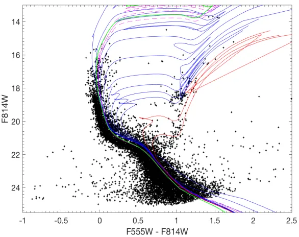
Figure 2.4: NGC 1711 color magnitude diagram (CMD) i.e.mF814W vs. mF555W F814W. Padova
isochrones are over plotted with blue lines representing isochrones of ages 20, 40, 80,100, 200, 400, 600, and 800 million years from top to bottom, and red lines represent 2 and 4 billion years. The isochrones in magenta correspond to the log (t/yr)=7.70±0.05. The solid
magenta line represents log (t/yr) = 7.70 i.e. approximately 50 million years and the dotted
magenta lines represent the upper and lower limit for the age of the cluster found by [7]. The isochrone corresponding to log (t/yr) = 7.70 ± 0.05 using MESA stellar tracks is plotted in
green. The cluster’s metallicity is taken to be -0.57 dex that corresponds to a Z=0.004.
interpolate the mass and luminosity values for the given age and metallicity of the cluster to obtain the MLR. During interpolation, we truncated some mass and luminosity values to make the relation monotonic for interpolation.
2.2 Mass Function
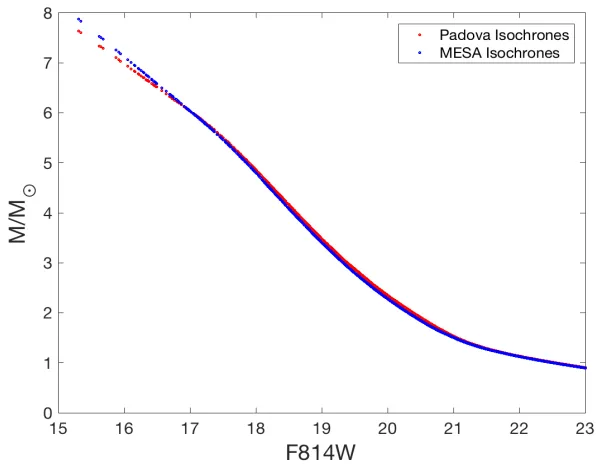
Figure 2.5: Theoretical mass-magnitude relations (MMR) for log (t/yr)= 7.70. The red line
represents the MMR obtained using Padova isochrones and the blue line represents the MMR using MESA isochrones. The respective ranges of masses obtained are (i) Padova: 0.90M to 7.63 M (ii) MESA: 0.89M to 7.87M .
2.3. MLPmodeling of theMassFunction 25
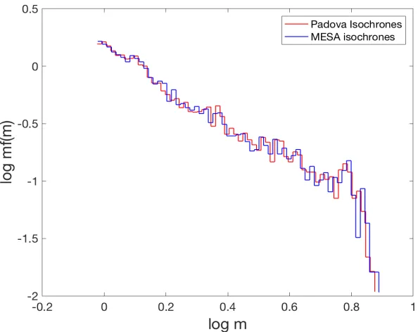
Figure 2.7: We have obtained the mass function for NGC 1711 using Padova and MESA isochrones. Logarithm of density is plotted as a function of mass in solar masses.
2.3 MLP modeling of the Mass Function
2.3.1 Fitting Results
The LM algorithm for the MLP function on the MF obtained from theoretical isochrones con-verges to the following set of parameter values that best represent a good fit (i) fit1 (Using Padova MLR): ↵0 = 1.72, µ0 = 0.09 and 0 = 0.02 and (ii) fit2 (Using MESA MLR):
↵0 = 1.77, µ0 = 0.08 and 0 = 0.01. The set of values shows physical meaning and below we discuss how their goodness of fit test statistics qualify the parameter values to be a good fit.
The first step to understanding how good the fit is to visually see whether the graph of the fitted MLP function on the observed MF lies close to all the data points. Statistically, a model is said to be a0good fit0 to the data: 1) if the assumptions of the least squares method are satisfied 2) if the coefficients of the model can be obtained with minimum uncertainty 3)
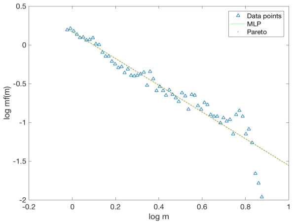
Figure 2.8: Using Padova isochrones: Mass function fitted with the MLP function. The plot above represents the graph for the best fit values ↵0 = 1.72, µ0 = 0.09 and 0 = 0.02. We obtained the same slope i.e. ↵+1=1.72 value for the Pareto function as well. The best Pareto fit is over plotted in a green colour.
2.3. MLPmodeling of theMassFunction 27
For fit 1 (Padova): ↵0 = 1.72, µ0 = 0.09 and 0 = 0.02 statistically, the residuals i.e. sum of squared errors (SSE) give a good indication whether the curve lies near the data points. The SSE value obtained for fit 1 is 1.25 which is low. We obtain anR2 value of 0.91 which explains variability in data. An R2 value closer to 1 indicates that a greater proportion of variance is accounted for by the model fit. We then look at the 95% of confidence bounds for each parameter. For↵0 =1.72, we have (1.58, 1.87) as the confidence interval,µ0 = 0.09 lies in (-0.15, -0.02) and 0 = 0.02 lies in (-0.07, 0.11). The narrowness of the 95% confidence intervals indicate that the coefficients of the model can be obtained with minimum uncertainty.
For fit 2 (MESA): ↵0 = 1.77, µ0 = 0.08 and 0 = 0.01,the SSE value obtained for is 1.34 which is low. We obtain anR2 value of 0.91. Confidence bounds for each parameter are: for ↵0 = 1.77, we have (1.62, 1.92), µ0 = 0.08 lies in (-0.15,-0.01) and 0 = 0.01 lies in (-0.16,0.19).
The best fit values are: Padova: ↵0 = 1.72, µ0 = 0.09 and 0 = 0.02 and MESA:
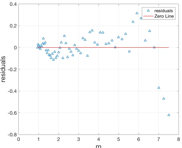
↵0 = 1.77, µ0 = 0.08 and 0 = 0.01 for M vs. log(f(m)). All data points lie near the best fitted curve of the MLP function and for the graph in log(M ), most data points lie closer to the curve for log(M )<0.8. Deviations above that limit are discussed in next section.
As discussed in section 2, in the limit 0 tending to 0 the MLP function behaves as a pure power-law distribution. We obtained 0= 0.02 for the Padova isochrones and 0= 0.01 for the MESA isochrones implying that the MLP takes power-law behaviour. This behaviour is seen graphically in Fig. 2.8 and Fig. 2.9. We also fitted the Pareto distribution function (equation 2) to the data points and found the slope to be same for the MF obtained from the Padova and MESA.
Figure 2.10: Residual plot for the best fit MLP function on the mass function obtained using Padova isochrones.
2.3. MLPmodeling of theMassFunction 29
the uncertainties are normally distributed [14]. A Q-Q plot, where Q stands for quantile, is a probability plot that compares if two distributions are similar or not. In the case of the error distribution, it compares with the standard normal distribution for which the points from the error distribution should lie on the straight liney= xcorresponding to the standard normal.
2.3.2 Truncated MLP
Figure 2.12: MF fitted with MLP function. The plot above represents the graph for the best fit values↵0 = 1.55,µ0= 0.08 and 0 = 0.07.
While deriving the pdf of the MLP distribution, Basu & Jones assumed an initial lognormal distribution with meanµ0and standard deviation 0. They then assumed an exponential growth of stellar masses because of accretion assuming a linear dependence on mass for the accretion rate i.e. dm
dt = m. This resulted the initial lognormal distribution to shift to a new meanµ0+ t
the distribution of lifetimes of accretion, with as the decay rate i.e. f(t)= e t, and obtained
the MLP function on integrating over infinite time. Accretion of mass onto the star for infinite time is not entirely physical because accretion is most likely stop at some maximum stopping time due to the dissipation of the surrounding gas. Thus, integrating equation 1.8 in the MLP derivation to a maximum stopping timeT, we obtained the truncated MLP:
Z T
0
1 p
2⇡ 0m
exp (ln m µ0 t)2
2 02 e
tdt
= ↵0
2 exp
⇣
↵0µ0+↵20 20/2
⌘
m (1+↵0)⇥
erf p1
2 ↵0 0
lnm µ0 T 0
!!
erf p1
2 ↵0 0
lnm µ0 0
!! !
(2.2)
Refer to Appendix A for derivation of equation above.
The truncated MLP function is a four-parameter pdf where µ0 and 0 describe the log-normal body,↵0 = / gives the slope of the power-law tail andT / 1 i.e. the maximum stopping time describes the truncation. Using the LM Algorithm, we found that the truncated MLP distribution follows a truncation when T = 2. The figure below shows the truncated
MLP probing the data points above 6 M when using the truncated MLP for a fixed stopping time for accretion. The reason for it being twice will be explored in a future work.
2.3.3 MLP as a hybrid
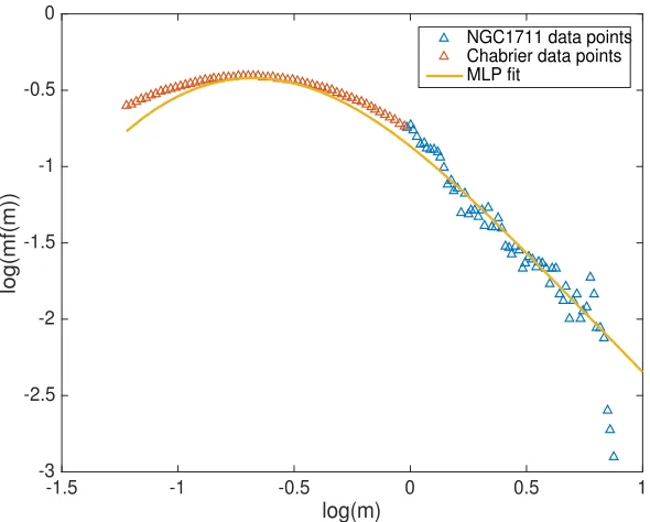
Another significant purpose of using the MLP distribution function is to check whether it can work as a hybrid to model both lognormal and power law behaviour as a single function. Since our data sample was complete only to mF814 = 23, we combined the NGC 1711 cluster data for theoretical MLR with an artificially generated data sample from the Chabrier lognormal functional form [4]. We generated an equal number (60) of data points in the range 0.06 M
2.3. MLPmodeling of theMassFunction 31
-1.5 -1 -0.5 0 0.5 1
log(m)
-3 -2.5 -2 -1.5 -1 -0.5 0
log(mf(m))
NGC1711 data points Chabrier data points MLP fit
to high mass stars. Then we again used the LM method on the combined data sample and obtained the best fitting MLP function with best fitting parameter values asµ0= 2.06±0.06,
0 =0.90±0.07, and↵0 = 1.57±0.13. Using the MLP properties [1], we found the mean of the distribution for the best fit parameter values to be 0.53 M . The mean for the NGC 1711 data points alone is 2.23M . The artificially generated data points provided a lognormal body to the distribution of NGC 1711 data points thus giving a higher sigma value 0 = 0.90 i.e. resulting in deviation from a pure-law behaviour. It also altered the mean of the distribution where the mean of the distribution now lies in the low mass end of the stellar regime. Our aim of joining the NGC 1711 data points with Chabrier data points was also to check whether the slope of the power-law tail is a↵ected by the lognormal body or not i.e. making the tail
steeper or shallower in logarithmic space. From our fitting results↵0 = 1.57±0.13 lies in the predicted interval of↵0 =1.72±0.14 for NGC 1711, hence showing not a significant e↵ect of the lognormal body on the slope of the power-law tail.
2.4 Summary
We derived MFs for the young and populous LMC stellar cluster NGC 1711 using two di↵erent
sets of theoretical isochrones. The slope and the mass range for the MF obtained seems to not depend on the underlying theoretical MLR. Using Padova we obtained the mass range of the MF to be 0.90 to 7.63M and using MESA we got the mass range as 0.89 to 7.87M .
We then investigated whether the MFs showed lognormal, power law or hybrid behaviour using the MLP function along with checking whether it can be adequately used to describe the MF of the stellar cluster. Since the MFs seems to be showing pure power law behaviour, the MLP function was able to give best fit parameter value for the slope of the MFs : (i) Padova:
↵0= 1.72±0.14 (ii) MESA:↵0 =1.77±0.15. In the limit where tends to 0, the MFs tend to a pure power-law behaviour. We obtained sigma values as (i) Padova: = 0.02 (ii) MESA:
2.4. Summary 33
because the data are limited tomF814 ¡ 23 . Since the data is only complete until 23 F814W apparent magnitude, we did not have many stellar masses less than 1M in our data set which is known to show lognormal behaviour in general.
The turnover at 6M is explored using a truncated MLP where we consider a fixed stopping time for accretion. The truncated MLP was able to probe the turnover giving evidence that accretion stops at a time scale analogous to the characteristic death time.
We also investigated whether the MLP function can model hybrid i.e. both lognormal as well as power law behaviour, and also to check whether adding a lognormal body to the data has any e↵ect on the slope of the power law tail. For that we generated artificial data points
from the Chabrier lognormal function [4] and combined the data points for NGC 1711 to get a complete data set with masses ranging over low, intermediate and high mass. We took the MF using Padova isochrones. We then again fitted the MLP function using a non-linear regression approach and obtained↵0 =1.57 which is less steep than the one obtained only for the fit on the cluster data i.e. ↵0 = 1.72, but lies in the predicted interval for↵0 =1.72 i.e. ↵0 =1.72±0.14. From this we can conclude the MLP can be used to model hybrid behaviour as a single function instead of using di↵erent functions with joining conditions. Our final conclusion is (i) NGC
[1] S. Basu, M. Gil, and S. Auddy. The MLP distribution: a modified lognormal power-law model for the stellar initial mass function. MNRAS, 449:2413–2420, May 2015.
[2] G Bertelli, A Bressan, Ci Chiosi, F Fagotto, and E Nasi. Theoretical isochrones from models with new radiative opacities. Astronomy and Astrophysics Supplement Series, 106, 1994.
[3] A. Bressan, P. Marigo, L. Girardi, B. Salasnich, C. Dal Cero, S. Rubele, and A. Nanni. PARSEC: stellar tracks and isochrones with the PAdova and TRieste Stellar Evolution Code. MNRAS, 427:127–145, November 2012.
[4] G. Chabrier. The Initial Mass Function: from Salpeter 1955 to 2005. In E. Corbelli, F. Palla, and H. Zinnecker, editors, The Initial Mass Function 50 Years Later, volume 327 ofAstrophysics and Space Science Library, page 41, January 2005.
[5] R. de Grijs, G. F. Gilmore, R. A. Johnson, and A. D. Mackey. Mass segregation in young compact star clusters in the Large Magellanic Cloud - II. Mass functions.MNRAS, 331:245–258, March 2002.
[6] R. de Grijs, R. A. Johnson, G. F. Gilmore, and C. M. Frayn. Mass segregation in young compact star clusters in the Large Magellanic Cloud - I. Data and luminosity functions.
MNRAS, 331:228–244, March 2002.
BIBLIOGRAPHY 35
[7] B. Dirsch, T. Richtler, W. P. Gieren, and M. Hilker. Age and metallicity for six LMC clusters and their surrounding field population. A&A, 360:133–160, August 2000.
[8] T. Lejeune and D. Schaerer. Database of Geneva stellar evolution tracks and isochrones for (UBV)J(RI)C JHKLL’M, HST-WFPC2, Geneva and Washington photometric
sys-tems. A&A, 366:538–546, February 2001.
[9] T. Maschberger and P. Kroupa. Estimators for the exponent and upper limit, and goodness-of-fit tests for (truncated) power-law distributions.MNRAS, 395:931–942, May 2009.
[10] M. Mateo. Main-sequence luminosity and initial mass functions of six Magellanic Cloud star clusters ranging in age from 10 megayears to 2.5 gigayears. ApJ, 331:261–293, August 1988.
[11] PC Myers. Growth of an initial mass function cluster in a turbulent dense core. The Astrophysical Journal Letters, 530(2):L119, 2000.
[12] B. Paxton, M. Cantiello, P. Arras, L. Bildsten, E. F. Brown, A. Dotter, C. Mankovich, M. H. Montgomery, D. Stello, F. X. Timmes, and R. Townsend. Modules for Experiments in Stellar Astrophysics (MESA): Planets, Oscillations, Rotation, and Massive Stars.ApJS, 208:4, September 2013.
[13] R. Sagar and T. Richtler. Mass functions of five young Large Magellanic Cloud star clusters. A&A, 250:324–339, October 1991.
[14] Achim Zielesny. From Curve Fitting to Machine Learning: An Illustrative Guide to Scientific Data Analysis and Computational Intelligence, volume 18. Springer Science &
Model Selection: Which Model to choose
for the IMF of Young Stellar Clusters?
Given the plethora of observational data on stellar mass distribution (IMF) in di↵erent
envi-ronments and many existing IMF models since the pioneering work of Salpeter [8] in 1955, it is important to study the statistical problem of model selection. Model selection aims to inves-tigate: which model can be used as the best approximating model to the underlying data set? One can use the Akaike Information Criterion (AIC) and the Bayesian Information Criterion (BIC) to do model selection for the set of di↵erent candidate models, given the data set. In this
chapter, we focus on the comparison of three candidate IMF models: the Modified Lognormal Power-Law (MLP) [2] probability distribution function, the Chabrier IMF [4] and the Kroupa IMF [5] using AIC and BIC, given the data set of stellar mass distribution in di↵erent
environ-ments.
To obtain the ranks for these three models on the basis of AIC/BIC, one first needs to
esti-mate the best fit parameters of these models on the underlying distribution. Even though one can estimate parameters of the functional forms by fitting models to the observed data us-ing a non-linear regression approach, this method involves numerical bias. Maiz Apellaniz & Ubeda showed that deriving the slope for the power-law functional form using a least-squares
3.1. Observational data 37
minimization method with uniform binning of data has significant numerical bias [7]. The cor-relation between the number of stars in each bin and the weights assigned to each bin causes the bias in the determination of the slope. Hence, we use the method of maximum likelihood for the estimation of parameters for the models which like the least-squares minimization approach aims to minimize the residuals by maximizing the likelihood function but is independent of the bias due to binning.
3.1 Observational data
(i) Orion Nebula Cluster (ONC): The stellar population has the mass range of 0.02M to 45.70
M . This mass range contains substellar, low, intermediate as well as high mass stars hence
has both a lognormal body and a power-law tail. Since the masses of the stars of the ONC population span over the entire mass regime, it is a perfect laboratory to test hybrid behaviour. (ii) NGC 1711: We obtain the mass range of 0.89 M to 7.84 M for the stellar population. This mass range spans some low mass stars but mostly intermediate and some high mass stars. It is useful to investigate power-law behaviour of the MF.
(iii) NGC 6611: The stellar population has mass range of 0.02M to 6.02M . The population spans over the substellar, low and intermediate mass regime but does not contain high mass stars. One can investigate the lognormal behaviour of the assumed SSP and probe some part of the power-law tail.
(iv) NGC 2024: The stellar population has the range of 0.02 M to 0.72 M .The population contains only substellar and low mass stars hence helps in modeling population distribution showing lognormal behaviour alone.
3.2 IMF Models and Parameter Estimation
(i) Chabrier functional form (Lognormal+ Power-law): this is a piecewise pdf having a
form on the intermediate and high mass regime i.e. above 1M [4, 3].
f(ln m)/
8 >>>>> < >>>>> : 1 p
2⇡ exp
" (ln m
µ)2
2 2
#
, m 1M
m ↵+1, m> 1M
(3.1)
The functional form of the lognormal distribution is given by:
f(m)= p 1
2⇡ mexp
" (ln m
µ)2
2 2
#
, m1M (3.2)
The lognormal function has two parameters: µand . The location parameterµis the mean
of the distribution and the scale parameter is the standard deviation of the distribution. The likelihood function of a lognormal distribution is given by:
L(µ, |mi)= N Y i=1 1 mi 1 p
2⇡ exp
" (ln m
µ)2
2 2
#
, (3.3)
Thus the parameters that maximize the likelihood function are given by:
ˆ
µ= X
k
ln mk
n , (3.4)
ˆ2 =X
k
(ln mk µˆ)2
n . (3.5)
(3.6)
The functional form of the Pareto distribution is given by:
f(m)= (↵ 1)a↵ 1m ↵, m>a, where↵ > 1and a > 0 (3.7)
↵ is the shape parameter for the distribution that determines the power-law tail while a is
be-3.2. IMF Models andParameterEstimation 39
haviour. The likelihood function for the Pareto distribution is given by :
L(↵|mi)= N
Y
i=1
(↵ 1)nan(↵ 1)min↵, (3.8)
Thus the parameter that maximizes the likelihood function is given by:
ˆ
↵= 1
"1 n
N
X
i=1
log(mai)
# 1
. (3.9)
(ii) Kroupa functional form (multi-segmented power-law): This is a piecewise pdf of a Pareto distribution, a Truncated-Pareto and a Power function. Essentially, they are all power-law distributions varying in either the sign of the exponent or whether they have an upper limit, lower limit or both.
f(ln m)/
8 >>>>> >>>< >>>>> >>>:
m↵1+1, m<0.08M ,where↵
1 > 1
m↵2+1, 0.08M m<0.50M , where↵
2 , 1
m ↵3+1, 0.50M m,where↵
3 > 1
(3.10)
The Pareto Function and Power Function represent the same distribution except↵< 1 for
Pareto and↵> 1 for Power Function. The parameter that maximizes the likelihood function
is given by equation 3.9. The best fit parameter value for the Truncated-Pareto distribution can only be obtained numerically by solving the following equation [10] :
¯
ln m= 1
ˆ ↵+1 +
b↵ˆ+1ln b a↵ˆ+1ln a
b↵ˆ+1 a↵ˆ+1 . (3.11)
whereais the lower limit of the distribution andbis the upper limit, anda 0 &b 0. (iii) MLP functional form: The functional form of the MLP is given by:
f(ln m)= ↵0
2 exp
⇣
↵0µ0+↵20 20/2
⌘
m ↵0⇥erfc p1
2 ↵0 0
lnm µ0 0
!!
Obtaining the best fit parameter that maximizes the likelihood function for the MLP is not possible analytically thus we undergo a global minimization search for lnL i.e. the negative log-likelihood function using simulated annealing.
The following tables give the best fitting parameter values for the di↵erent stellar
popula-tions. MBr, MBr1 andMBr2 represent the respective joining points.
Data µ ↵ MBr
ONC -1.54 0.54 2.46 1M
NGC 1711 -0.71 0.65 2.92 1M
NGC 1711 - - 2.90 0.89M
NGC 6611 -0.32 0.65 3.89 1M
NGC 2024 -2.06 1.0 - 1M
Table 3.1: Best fit parameter values for the Chabrier functional form.
Data ↵1 ↵2 ↵=↵3 MBr1 MBr2 ONC 3.20 0.02 2.18 0.08 0.50
NGC 1711 - - 2.90 - 0.50
NGC 1711 - - 2.90 - 0.89
NGC 6611 0.88 0.37 3.52 0.08 0.50 NGC 2024 0.32 -1.22 5.03 0.08 0.50
Table 3.2: Best fit parameter values for the Kroupa functional form.
Data µ ↵=↵0+1
ONC -2.01 0.35 2.42
NGC 1711 -0.11 0 2.90
NGC 6611 -0.97 0.98 4.59 NGC 2024 -2.26 0.98 max
Table 3.3: Best fit parameter values for the MLP functional form.
Note that: dNdm /m ↵while dN
3.2. IMF Models andParameterEstimation 41
Figure 3.1: Logarithm of f(ln m) is plotted as a function oflog(m/M ) for the Orion Nebula Cluster.
Figure 3.2: Logarithm of f(ln m) is plotted as a function of log(m/M ) for the cluster NGC
Figure 3.3: Logarithm of f(ln m) is plotted as a function of log(m/M ) for the cluster NGC
6611.
Figure 3.4: Logarithm of f(ln m) is plotted as a function of log(m/M ) for the cluster NGC
3.3. ModelSelection usingInformationCriterion 43
3.3 Model Selection using Information Criterion
The Chabrier IMF [4] i.e. lognormal + power-law functional form and the Kroupa IMF [5]
i.e. the mutli-segmented power-law functional form are the two most commonly used IMF models up-to-date. Even though these two models can be adequately used to study the features and characteristics of the stellar mass distribution i.e. the lognormal body and the power-law tail, they require di↵erent joining conditions that add to the number of free parameters; this
in return increases the complexity of these models. MLP on the other hand is a pdf of only 3 parameters that can probe both the lognormal body and the power-law tail of the MF as a single function (refer to Chapter 2).
The AIC or the BIC provide a trade o↵ between how well the model fits the data and how
complex the model is. Comparing the Chabrier, Kroupa and the MLP distribution functions on the basis of the ranks obtained using the AIC/BIC will help us find the simplest model of the
competing models i.e. a model with the least number of parameters but also the one that lies very close to the data set.
We compute the AIC value by AIC = 2ln L+ 2k where L is the value of the likelihood
function maximized by the best fit parameters andkis the number of parameters in the model [1]. The model with the minimum AIC value gives us the best model amongst the candidate set of models.
The model with the minimum BIC value also gives us the best approximating model. BIC is defined as BIC = 2ln L + k ln N where N is the number of data points [9]. The only
di↵erence between AIC and BIC is that BIC has a more strict condition to penalize a model for
overfitting. The penalty term in the AIC is 2kwhile in the BIC penalty term isk ln N. For large data sets, AIC can tend to pick models with more number of parameters than the true model while BIC penalizes an overparameterized model for large data sets with a stronger penalty term [6].
For models that have similar AIC value, we find the relative likelihood and the associated Akaike weight for the model. The relative likelihood for the model is given byexp(AICmin AICi
whereAICmin is the lowest AIC rank for all the models,AICi are the individual AIC ranks for
the candidate model and AICi is the di↵erence. Akaike weight is given by PAICAICmin AICi
min AICi. A higher Akaike weight tells us that the model has the most probability to be the best fit model amongst the candidate models.
The joining conditions for the Chabrier IMF and the Kroupa IMF are kept fixed as 1M for Chabrier and 0.08M and 0.50M respectively. The other are kept as free parameters.
Model parameters -2 ln L AIC BIC AICi Relative likelihood Akaike weight
Chabrier 3 7600.3 7606.1 7623.7 2209.8 0 0
Kroupa 3 8696.4.0 8702.4 8719.9 330.61 0 0
MLP 3 5390.3 5396.3 5413.8 0 1 1
Table 3.4: Negative likelihood function values, AIC and BIC for the ONC.
Model parameters -2 ln L AIC BIC AICi Rel. Like. Akaike weight
Chabrier (1M ) 3 6491.8 6497.8 6517.6 2644.3 0 0
Chabrier (0.89M ) 3 3847.5 3853.5 3873.3 0 1 0.33
Kroupa (0.50M ) 3 11957 11963 11983 8109.5 0 0
Kroupa (0.89M ) 3 3847.5 3853.5 3873.3 0 1 0.33
MLP 3 3847.5 3853.5 3873.3 1 0.97 0.32
Table 3.5: Negative likelihood function values, AIC and BIC for the NGC 1711.
Model parameters -2 ln L AIC BIC AICi Relative likelihood Akaike weight
Chabrier 3 1222.0 1228.0 1239.6 194.91 0 0
Kroupa 3 1141.9 1147.9 1159.6 114.8 0 0
MLP 3 1027.1 1033.1 1044.7 0 1 1
3.4. Discussion 45
Model parameters -2 ln L AIC BIC AICi Relative likelihood Akaike weight
Chabrier 3 196.69 202.69 209.39 0 1 0.36
Kroupa 3 197.19 203.19 209.89 0.50 0.77 0.28
MLP 3 196.76 202.76 209.46 0.07 0.96 0.35
Table 3.7: Negative likelihood function values, AIC and BIC for the NGC 2024.
3.4 Discussion
The aim of the study is to provide a quantitative/statistical analysis of the comparison of di↵
er-ent IMF models for stellar populations with di↵erent mass regimes. These MFs of the stellar
populations show di↵erent behaviour depending on the range of the masses obtained.
The MF of ONC shows hybrid behaviour i.e. both a lognormal as well as power-law be-haviour. On computing the negative log-likelihood, the AIC and the BIC value, one can con-clude that the MLP is the best approximating pdf to model hybrid behaviour of the MF as compared to Chabrier IMF with a fixed breaking point at 1 M or the Kroupa IMF with fixed breaking points as 0.08 M and 0.50 M . The MLP had the lowest value for the negative log-likelihood thus showing that the model lies closer to the data than the other two models. The best fit parameters obtained for the ONC using the MLP are↵0 = 1.42,µ0 = 2.014 and
0 =0.35. Thus the best fit value for the↵=↵0+1 fordN/dlnm/ m ↵+1obtained is 2.42.
The MF of NGC 1711 shows pure power-law behaviour, even though it has some low mass stars upto 0.89 M . MLP, Chabrier IMF with breaking point 0.89M instead of 1M and Kroupa IMF with breaking point 0.50M gave the same negative log-likelihood value. The best fit parameter for the↵fordN/dlnm / m ↵+1 is 2.90 for masses above 0.89M . The Chabrier IMF, the Kroupa IMF and the MLP had similar Akaike weights hence all three models are ranked equally.
the joining condition fixed as 1 M which is why the model departs away from the underlying data points. For the cluster NGC6611, we get the lowest AIC value for the MLP function. Best fit parameters obtained are↵0 =4.6,µ0 = 0.97 and 0 =0.98.
The MF of NGC 2024 shows pure lognormal-like behaviour. We obtained the lowest neg-ative log-likelihood value for both the Chabrier and the MLP function. On the plot for the MF of NGC 2024, the Chabrier and the MLP overlap each other. The best fit parameters obtained are µ0 = 2.26 and 0 = 0.98. ↵0 took the value of the upper limit of the bound constraint while optimizing the negative log-likelihood function for the MLP. This showed that the data set followed pure-lognormal behaviour in the limit of↵becoming too large, the MLP becomes a lognormal distribution.
In general on the basis of AIC and BIC, one can statistically infer that the MLP is the best approximating model to the mass distribution of underlying stellar populations having di↵erent