ABSTRACT
MACINTOSH, CHRISTOPHER WILLIAM. The 6 May 2010 Elevated Supercell During VORTEX2. (Under the direction of Matthew Parker.)
Convection over statically stable boundary layers (i.e., elevated convection) occurs over
much of the United States, producing heavy rainfall, hail, and occasionally severe surface
winds. Much of the current literature on elevated convective storms concerns those of a
linear morphology; studies of elevated supercells are largely absent. Elevated supercells
present an operational challenge because they look similar to surface-based storms on radar,
which can lead forecasters to issue warnings for severe winds and tornadoes that are not
likely to occur. However, severe winds do seem to occur in a handful of elevated supercells,
but the reasons behind their formation are currently unknown. To further understand the
governing dynamics, an elevated supercell case from the second Verification of the Origins
of Rotation in Tornadoes Experiment (VORTEX2) on 6 May 2010 is investigated.
VORTEX2 measurements provide an unprecedented dataset that includes radar data from
Doppler-on-Wheels (DOW) and Shared Mobile Atmospheric Research and Teaching Radar
(SMART-R) mobile radars and surface mobile mesonets. Observations show that the
supercell formed over a stable inversion and was decoupled from the surface. As a result of
the decoupling, the surface cold pool was fueled without the help of mid-level air. Wave-like
structures also appeared to be present in the low-levels, showing up as banded reflectivity
structures moving perpendicular to the storm motion. Additionally, idealized modeling using
a sounding from this case is used to clarify the structure and maintenance of this supercell as
AGL where instability was present. These parcels reached their LFCs due to the supercell's
own dynamic lifting with some possible assistance from gravity waves that were present in
the environment; both of these mechanisms likely maintained the main updraft throughout its
life. Below ~1.2 km AGL, air followed an “up-down” trajectory, being lifted dynamically
before becoming strongly negatively buoyant and descending quickly back to the surface.
Up-down parcels originating in the lowest 100 m were the driver behind severe surface
winds, leading to downdrafts that spread out upon reaching the ground and were further
© Copyright 2014 by Christopher William MacIntosh
The 6 May 2010 Elevated Supercell During VORTEX2
by
Christopher William MacIntosh
A thesis submitted to the Graduate Faculty of North Carolina State University
in partial fulfillment of the requirements for the Degree of
Master of Science
Marine, Earth, and Atmospheric Sciences
Raleigh, North Carolina
2014
APPROVED BY:
_____________________________ _____________________________
Sandra Yuter Gary Lackmann
_____________________________ Matthew Parker
ii
DEDICATION
iii
BIOGRAPHY
Chris MacIntosh grew up in St. Charles, MO. As a young'n, he was always frightened, but
eventually intrigued, by storms. He can recall one instance growing up where he saw his
neighbor's gutter twisted and ripped from their house by strong winds that made him sure that
he wanted to study meteorology. Chris also admits that the movie Twister may have played a
role in his choice for a career.
He graduated with a Bachelor of Science in Meteorology from Iowa State University in
May of 2012. At ISU, he had many opportunities to storm chase and fuel his passion for
insane weather, covering ten states and observing numerous tornadoes over four years.
During his final two years at Iowa State, Chris had the opportunity to work as a research
assistant to Dr. William Gutowski, post-processing data for the North American Regional
Climate Change Assessment Program (NARCCAP) that first allowed him to be a part of a
true research environment and piqued his curiosity towards graduate school. He was also a
volunteer with the Tactical Weather Instrumented Sampling in/near Tornadoes Experiment
(TWISTEX) in the summer of 2011, cementing his interest in severe weather research and
iv
ACKNOWLEDGEMENTS
I would like to first thank all of my family and friends that have supported and encouraged
the pursuit of my dreams throughout the years. My advisor, Dr. Matthew Parker, also
deserves an immense amount of thanks for all of his assistance over the last two years.
Furthermore, I would also like to thank my committee members, Drs. Sandra Yuter and Gary
Lackmann, as well as the members of the Convective Storms Group (CSG) at NCSU for their
help along the way. Finally, I want to acknowledge Casey Davenport for her guidance on the
v
TABLE OF CONTENTS
List of Figures ... vi
Chapter 1 Introduction ... 1
1.1 Background ... 1
1.2 Motivation ... 5
1.3 Outline of Thesis ... 6
Chapter 2 Observations of 6 May 2010 ... 11
2.1 VORTEX2 Observational Platforms and Methods... 11
2.2 Observations ... 13
2.2.1 Evolution of pre-convective environment ... 13
2.2.2 Supercell observations ... 15
2.2.3 Observational summary ... 19
Chapter 3 Numerical Model Simulations ... 41
3.1 Model Setup ... 41
3.2 Control Simulation ... 44
3.3 Simulation Summary ... 50
Chapter 4 Conclusions and Future Work ... 72
vi
LIST OF FIGURES
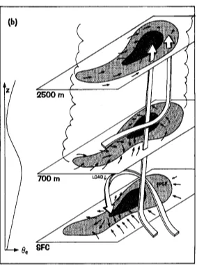
Figure 1.1 Conceptual model of a nighttime mesoscale convective system. Large arrows represent the updraft and downdraft branches of the system. Vertical profile of θe is shown at the left. Reproduced from Bernardet and
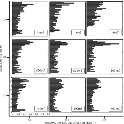
Cotton (1998). ... 7 Figure 1.2 4 km updraft parcel origin for various stable layer simulations. The labels
(i.e., “100mC”) represent the depth of the stable layer (i.e., “100m”) and lapse rate classification (“C” is the largest at -21.5 K km-1). Reproduced from Nowotarski et al. (2011). ... 8 Figure 1.3 As in Fig. 1.2, but for 2 km downdraft parcel destinations. Reproduced
from Nowotarski et al. (2011). ... 9 Figure 1.4 Conceptual model of circulation around a material circuit in an
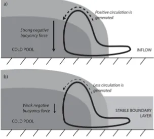
environment (a) without a stable layer and (b) with a stable layer. Reproduced from Nowotarski et al. (2011). ... 10
Figure 2.1 Dual-Doppler lobes for DOW6 and SMART-R2. Radar from KGLD WSR-88D is shown at 0057 UTC 7 May 2010. Radar locations are marked with red circles. StickNets were located every 8 km along the dashed purple line. ... 21 Figure 2.2 NAM analyses of isotachs (kts; shaded), wind observations, and heights
(dm) at (a,c) 250 mb and (b,d) 500 mb at (top row) 1200 UTC 6 May 2010 and (bottom row) 0000 UTC 7 May 2010. ... 22 Figure 2.3 RAP surface observations at (a) 1207, (b) 1807, (c) 2207 UTC 6 May
2010, and (d) 0007 UTC 7 May 2010. Approximate locations of the low pressure systems (‘L’), dryline (brown line), and cold (blue line) and warm (red line) fronts are also shown... 23 Figure 2.4 Locations where soundings were launched on 6 & 7 May 2010. Pre-storm
soundings (top) at 1745 and 2053 UTC 6 May 2010 are indicated by an open circle and cross, respectively, and the approximate location of the warm front at 2000 UTC 6 May 2010 is shown by the red line. Radar imagery from the KGLD WSR-88D nearest in time to the launch is shown in the 0039, 0106, and 0117 UTC 7 May 2010 plots with the sounding location indicated by a cross. ... 24 Figure 2.5 Skew-T/log-p plot of upper-air soundings and hodographs (a) north of the
warm front at 1745 UTC 6 May 2010 and (b) south of the warm front at 2053 UTC 6 May 2010. Wind barbs are in knots. ... 25 Figure 2.6 (a) MUCAPE (J kg-1) and (b) 0–6 km bulk shear (m s-1) at 2200 UTC 6
May 2010. Both parameters are from the SPC mesoanalysis archive. ... 26 Figure 2.7 Reflectivity (dBZ) from the Goodland, KS (KGLD) WSR-88D radar
vii
red line is the approximate location of the warm front. ... 27 Figure 2.8 Skew-T/log-p plot of upper-air soundings and hodographs in the (a)
near-inflow of the target storm at 0039 and (b) far-near-inflow at 0106, and (c) near the forward-flank at 0117 UTC 7 May 2010. ... 28 Figure 2.9 Vertical profiles of CAPE (J kg-1), CIN (J kg-1), and delta-z (m) for the
(blue) 1745 and (red) 2053 UTC 6 May 2010 and (green) 0039, (purple) 0106, and (orange) 0117 UTC 7 May 2010 soundings. The parameter
delta-z is the vertical distance a parcel would need to be lifted to reach its level of free convection (LFC). ... 29 Figure 2.10 Reflectivity (dBZ) and radial velocity (m s-1) at 1.3˚ from SMART-R2 at
(a,b) 0045:14, (c,d) 0051:14, (e,f) 0057:14, and (g,h) 0103:14 UTC 7 May 2010. Dashed (dotted) lines in radial velocity data mark the approximate location of convergence (divergence). ... 30 Figure 2.11 Reflectivity (dBZ) and radial velocity (m s-1) from SMART-R2 at (a,b)
5.6˚ at 0045:53, (c,d) 7.8˚ at 0046:18, (e,f) 10.0˚ at 0046:32, and (g,h) 11.4˚ at 0046:45 UTC 7 May 2010. Approximate location of the mid-level mesocyclone is circled. Height of mesocyclone is labeled on each velocity image. ... 31 Figure 2.12 Reflectivity (dBZ) from SMART-R2 at (a) 4.9˚ at 0039:51, (b) 4.9˚ at
0051:51, (c) 4.2˚ at 0100:45, (d) 3.5˚ at 0109:39, (e) 3.5˚ at 0118:33, and (f) 2.7˚ at 0127:49 UTC 7 May 2010. Snapshots were taken when the hook echo was at a height of ~2.5 km. ... 32 Figure 2.13 Reflectivity (dBZ; shaded), vertical velocity greater (less) than 3 (-3) m s
-1
(contoured in purple, negative values dashed), and storm-relative wind vectors at 0.5, 1.0, 1.5, 2.0, 2.5, and 3.0 km AGL from a dual-Doppler analysis using DOW6 and SMART-R2 at 0058 UTC 7 May 2010. Positions are relative to the location of SMART-R2 in km. ... 33 Figure 2.14 Reflectivity (dBZ) and radial velocity (m s-1) from SMART-R2 at 4.2˚ at
(a,b) 0039:40, (c,d) 0043:02 and (e,f) 0045:40. Arrows indicate anticyclonic rotation... 34 Figure 2.15 Reflectivity (dBZ) and radial velocity (m s-1) from DOW6 at 0.5˚ at (a,b)
0110:28, (c,d) 0112:01, (e,f) 0112:57, and (g,h) 0114:50 UTC 7 May 2010. Wave locations are indicated by ellipses. ... 35 Figure 2.16 Reflectivity (dBZ) and radial velocity (m s-1) from SMART-R2 at 1.3˚ at
(a,b) 0051:14, (c,d) 0054:35, (e,f) 0057:14, and (g,h) 0100:19 UTC 7 May 2010. Solid black line indicates radial used in Fig. 2.19. Dashed (dotted) lines in radial velocity data mark the approximate location of convergence (divergence). ... 36 Figure 2.17 Velocity (m s-1) and reflectivity (dBZ) along a radial from SMART-R2 at
viii
Figure 2.18 Reflectivity (dBZ; shaded) from DOW6/DOW7 dual-Doppler synthesis and time-to-space converted mobile mesonet and StickNet observations of storm-relative surface winds and (a) θ and (b) θe in K at 0113 UTC 7
May 2010. Tracks are 3 minutes in length. Positions are relative to the location of DOW6 in km. A vertical profile of θe (K) from the 0117 UTC
7 May 2010 sounding (Fig. 2.5c) is included along the right side for reference. ... 38 Figure 2.19 Reflectivity (dBZ) from the Hastings, NE WSR-88D Doppler radar
(KUEX) at (a) 0204:32, (b) 0300:12, (c) 0400:35, and (d) 0501:00 UTC 7 May 2010. Hill City and Russell, KS are marked with a star and ‘X’, respectively. Target supercell in the study is highlighted by an ellipse. ... 39 Figure 2.20 Peak 5 sec wind gusts (knots) from the ASOS stations at Russell, KS
(RSL; blue) and Hill City, KS (HLC; red) from 0000-0900 UTC 7 May 2010... 40
Figure 3.1 (a) Skew-T/log P plot of the model sounding (blue) compared to the thermal profiles of the 0039 (green) and 0117 UTC (red) 7 May 2010 soundings and hodograph of the 0106 UTC (magenta) 7 May 2010 sounding. (b) CAPE, CIN, and delta-z vertical profiles for the model, 0039, and 0117 UTC 7 May 2010 soundings. Colors are the same as in (a). Delta-z is the distance a parcel is required to be lifted to reach its LFC. ... 52 Figure 3.2 Plan views of reflectivity (shaded; dBZ), ground-relative wind vectors,
and vertical velocity greater (less) than 5 (-5) m s-1 120 min into the simulation at 0.5, 1.0, 1.5, 2.0, 2.5, 3.0 km AGL. The potential temperature deficit at the surface is shown with the 0.5 km AGL reflectivity (contoured in dashed blue at -1 and -3 K). ... 53 Figure 3.3 As in Fig. 3.2, but 180 min into the simulation. ... 54 Figure 3.4 Plan views of tracer concentration (shaded) and vertical velocity every 10
m s-1 (purple) 120 min into the simulation at 5 km AGL. Tracer originates in the 0.05–0.5, 0.5–1.0, 1.0–1.5, 1.5–2.0, and 2.0–2.5 km layers with a maximum concentration of 1. The 35 dBZ contour is shown in black for reference. ... 55 Figure 3.5 Normalized origins of updraft parcels in 100 m deep layers 120 min into
the simulation (or 30 min after model restart). Updraft parcels were defined as those with w ≥ 10 m s-1 at 5 km and above in a box centered around the storm. ... 56 Figure 3.6 Average updraft (black) and up-down (white) trajectories near the main
updraft. Potential temperature deficit (shaded; K) was averaged from y =-20 to -10 km at t = 1=-20 min. Boxes on trajectories represent the parcel’s location 120 min into the simulation. ... 57 Figure 3.7 Height (black; m) and (left) dynamic vertical acceleration (red; m s-2) and
ix
average up-down parcels originating in the 0.00–0.25, 0.25–0.50, 0.75– 1.00, and 1.00–1.25 km AGL layers. ... 58 Figure 3.8 Box-and-whisker plots for the average updraft (left) and up-down (right)
parcels of (a) maximum vertical velocity, (b) maximum vertical vorticity, and (c) maximum vertical vorticity... 59 Figure 3.9 Parcel trajectory (black) and vorticity vectors (teal) for the (a) average
up-down parcel originating in the 0.75-1.00 km AGL layer and (b) average mesocyclone parcel originating in the 2.00–2.25 km AGL layer. ... 60 Figure 3.10 (a) Height (m) and (b) vertical vorticity (s-1) over time along average
mesocyclone parcels originating in the 1.00–1.25 (green), 1.00–1.25 (yellow), 1.25–1.50 (light orange), 1.50–1.75 (orange), 1.75–2.00 (dark orange), 2.00–2.25 (light red), 2.25–2.50 (red), 2.50–2.75 (dark red), and 2.75–3.00 km (fuchsia) layers. ... 61 Figure 3.11 (a) Height (m), (b) dw/dz (s-1), and (c) vertical vorticity (s-1) over time
along average up-down parcels originating in the 0.00–0.25 (purple), 0.25–0.50 (blue), 0.75–1.00 (aqua), and 1.00–1.25 km (green) layers. ... 62 Figure 3.12 (a) Plan view of vertical vorticity (shaded; s-1), vertical velocity ≤ -3 m s-1
(hatched), and the 35 dBZ contour of reflectivity (thick black line) and (b) x-z cross-section of averaged vertical vorticity (shaded; s-1) and vertical velocity ≤ -3 m s-1
(hatched). An averaged up-down parcel trajectory near the hook echo is shown in pink. Quantities in (b) were averaged between y = -14 and -6 km. ... 63 Figure 3.13 (a) Height (black; m) and dynamic vertical acceleration (red; m s-2), (b)
height (black) and buoyant vertical acceleration (blue; m s-2),(c) height (black) and vertical vorticity (purple; s-1), and (d) vertical velocity (green; m s-1) and vertical vorticity (purple) over time for an averaged up-down hook that descended behind the hook echo (pink trajectory shown in Fig. 3.12). ... 64 Figure 3.14 Vertical cross-sections through the (a) short and (b) long axis of the
supercell updraft of buoyancy with storm-relative wind vectors, buoyant pressure perturbations with buoyant acceleration vectors, and dynamic pressure perturbations with dynamic acceleration vectors 120 min into the simulation. w ≥ 5 m s-1 is shaded in gray and vertical accelerations ≥ 0.05 m s2 are hatched in red. Buoyancy is contoured every 0.10 m s2 and the pressure perturbations are contoured every 50 Pa with negative values dashed. ... 65 Figure 3.15 x-z cross sections of w (shaded; m s-1), potential temperature (K), and
ground-relative wind vectors 120, 140, 160, and 180 min into the simulation. ... 66 Figure 3.16 As in Fig. 3.14, but for the (a) short and (b) long axis of the downdraft. w
≤ -5 m s-1
x
deficit (shaded; K) (top) 120 and (bottom) 180 min into the simulation. The 35 dBZ contour is shown in black for reference. The vertical profile of base state equivalent potential temperature (K) is shown on the right. ... 68 Figure 3.18 Normalized destinations of downdraft parcels originating above 1 km
AGL 120 min into the simulation (or 30 min after restart). Downdraft parcels were defined as those with w ≤ -3 m s-1 in the lowest 2 km AGL at any point during their life and were then sorted to only include those that originated above 1 km AGL. ... 69 Figure 3.19 (a) Ground-relative wind magnitude (shaded; m s-1) and cold pool
(dashed; contoured at -1 and -3 K) at the surface with parcels associated with this wind maximum in black (parcel #20) and grey (parcel #220). (b) Vertical cross-section of dynamic pressure perturbations (shaded; Pa), storm-relative wind vectors, and parcel trajectories as in (a). Pressure perturbations were averaged over lat = -12 to -2. Both plots are from 123 min into the simulation. ... 70 Figure 3.20 (a,e) Height (black; m) and dynamic vertical acceleration (red; m s-2),
1
Chapter 1
Introduction
1.1
Background
On 6 May 2010, the second Verification of the Origins of Rotation in Tornadoes Experiment
(VORTEX2; Wurman et al. 2012) armada sampled a storm that was believed to be an
elevated supercell1, compiling an unprecedented dataset over a variety of observational
platforms. Elevated supercells are rarely sampled during field projects, since the objectives of
the experiment typically lie elsewhere2. The case used in this study was the first storm to be
sampled during the 2010 session of VORTEX2 and was a “shakedown” case for many of the
instruments and mobile Doppler radars. Even so, the novelty of the target storm makes it a
dataset worth studying.
The definition of convection that is considered to be elevated varies by author (Colman
1990a; Corfidi et al. 2008; Parker 2008; Nowotarski et al. 2011). Occasionally, convection
may appear elevated even though some parcels continue to be lifted from the near-surface
layer. Generally, it is only in environments with extreme static stability and/or zero
surface-based convective available potential energy (CAPE) that storms are completely elevated; if
these qualifications are not met, we consider the storm to be surface-based. In other words,
1
A supercell is a thunderstorm with a rotating updraft (e.g., Lemon and Doswell 1979). A storm is generally considered to be elevated when it is only ingesting inflow parcels from above the near-surface layer.
2
2
the definition of elevated convection used in the present study requires convection to receive
all of its inflow parcels from above the near-surface layer in an environment without
surface-based CAPE. The majority of previous studies of elevated convection focused on mesoscale
convective systems (MCSs). Thus, most of what is known about elevated convection, its
environment, and the relevant processes may actually be specific to elevated MCSs.
Although elevated convective environments possess near-zero surface-based CAPE,
appreciable instability is present aloft (Colman 1990a,b; Grant 1995; Moore et al. 1998;
Thompson et al. 2003; Horgan et al. 2007). Nocturnal boundary layers (e.g., Marsham et al.
2011), frontal inversions (e.g., Colman 1990a), or outflow from previous convection
(Carbone et al. 1990) are the typical sources for the stable layer near the surface with storms
either forming on top of or translating over the stable air mass. For a storm to form over a
stable layer, parcels with instability aloft need to be lifted to their levels of free convection so
that the elevated instability can be released. This can be accomplished, for instance, by
frontal lifting (e.g., Moore et al. 1998), interactions between gravity currents and pre-existing
boundaries (e.g., Carbone et al. 1990), or lifting by density currents, bores, and gravity waves
(e.g., Rotunno et al. 1988; Koch and Clark 1999; Marsham and Parker 2006; Morcrette et al.
2006; Ziegler et al. 2010; Marsham et al. 2011). The lifting mechanism likely differs on a
storm-by-storm basis and depends on micro-, meso-, and synoptic-scale features.
After initiation, elevated convective systems may be maintained by the aforementioned
lifting mechanisms with further support from the advection of high theta-e air by a low-level
jet (Bernardet and Cotton 1998). In stable environments, Raymond and Rotunno (1989)
3
enough to produce an outflow that propagates faster than the gravity waves in the stable
layer. Cold pool lifting could potentially be enhanced if gravity waves stay in phase with
convective updrafts (i.e., co-location of upward motion; Schmidt and Cotton 1990) or if the
cold pool propagation speed and vertical wind shear are balanced (Rotunno et al. 1988).
However, it is not clear that surface cold pools occur in many elevated systems. It is possible
that this cold outflow could be produced prior to stabilization (e.g. Parker 2008; Ziegler et al.
2010) or in situ cooling of the stable layer could occur if relative humidity is suitably low.
Alternatively, Bryan and Weisman (2006) identified the presence of an elevated cold pool
(2–4 km layer) above a stable layer, which worked to continually release elevated instability
by lifting air along its leading edge. Bores may also provide sufficient lift to sustain elevated
convection; Parker (2008) found in his idealized simulations of MCSs in environments with
low-level cooling that as the convection became elevated, a “gravity-wave-like bore”
maintained the convective updrafts. For supercells, the enhanced vertical perturbation
pressure gradient acceleration due to the presence of environmental shear and to rotation in
the midlevels (Klemp 1987; Weisman and Rotunno 2000) has also been shown to help
maintain elevated convection above stable layers (Billings and Parker 2012). It is possible
that storm maintenance mechanisms vary from case to case even for a given storm type.
Heavy precipitation (with associated flash flooding) and large hail are seemingly the
most common hazards associated with elevated convection (e.g., Grant 1995; Moore et al.
1998; Horgan et al. 2007), but severe surface winds have also been observed on a limited
basis (e.g., Grant 1995; Schmidt and Cotton 1989; Bernardet and Cotton 1998; Bryan and
4
convection are somewhat mysterious with various studies concluding that different
storm-scale and mesostorm-scale processes were most important. It has long been presumed that
downdrafts of elevated storms cannot penetrate through a stable layer to the surface (e.g.,
Kuchera and Parker 2008). Parcels are thought to be slowed in their descent to the surface
due to the reduction of negative buoyancy, presumably reducing the severe threat. In
contrast, Schmidt and Cotton (1989) and Bernardet and Cotton (1998) both saw “up-down”
trajectories (Fig. 1.1) associated with severe downdrafts in an elevated squall line and an
elevated derecho, respectively. In such cases, parcels in the stable layer initially rise upward
due to an upward-directed vertical perturbation pressure gradient. This ascent, in turn, causes
these parcels to become strongly negatively buoyant and descend rapidly back to the surface.
Both studies found that the resulting surface winds exceeded severe criteria due to
acceleration of the flow by the horizontal pressure gradient in the stable layer. Knupp (1996)
also reported “up-down” trajectories associated with the downdrafts of a
microburst-producing storm in Colorado. In this case, inflow air was slightly stabilized under the
presence of an echo overhang (anvil shading), causing somewhat negatively buoyant air to be
lifted over the cold pool, become more negatively buoyant, and descend rapidly to the
surface.
As mentioned previously, the majority of studies on elevated convection have been
focused on mesoscale convection systems; however, Nowotarski et al. (2011) attempted to
tackle the problem of elevated supercells by using a numerical model to compare
surface-based supercells to those over stable boundary layers. The authors were intrigued by the
5
Kis and Straka (2010). Billings and Parker (2012) studied several nocturnal
tornado-producing storms they originally presumed to be elevated, but they ultimately concluded they
were likely ingesting air from the near-surface layer and were not elevated by definition.
Interestingly, the simulated “elevated” supercells in the Nowotarski et al. (2011) study were
still fueled by parcels from the near-surface layer, except in the case of extreme stability (Fig.
1.2). In addition, mid-level downdrafts were only unable to reach the surface in the case of
extreme stability (Fig. 1.3). At the surface, weaker convergence and baroclinic vorticity
generation were found by Nowotarski et al. (2011), leading to weaker near-surface vertical
vorticity (Fig. 1.4). This is one possible reason for the apparent hindered tornado potential in
elevated supercells. Notably, the Nowotarski et al. (2011) study used statically stable
boundary layers; in contrast, the 6 May 2010 VORTEX2 case exhibited a well-mixed
boundary layer, which was capped by a temperature inversion and had no CAPE. Such subtle
differences are potentially quite important operationally, since supercells have comparable
values of vertical vorticity and vertical velocity in the mid-level mesocyclone to those in
surface-based supercells and are arguably indistinguishable from surface-based storms on
radar. Thus, a nowcasting problem emerges, since operational radars often overshoot the
stable surface layer beneath elevated convection. It is therefore difficult to determine the
likelihood that an elevated storm is producing a tornado or severe surface winds.
1.2
Motivation
6
research known to the author; it is no wonder why so little is understood about these storms.
Although a number of plausible dynamical hypotheses have been advanced in the
aforementioned research, many questions remain unanswered. How are parcels with
appreciable instability lifted to their levels of free convection? How is this lifting maintained
throughout the storm’s existence? How does the stable layer influence the structure and
maintenance of an elevated storm? What is the mechanism behind severe surface wind
production in the presence of a stable layer? And, do the answers to these fundamental
questions vary among storm types? Observations and idealized numerical modeling will be
exploited to determine and explain the processes supporting the structure, maintenance, and
severe surface wind production of the 6 May 2010 elevated supercell from VORTEX2.
1.3
Outline of Thesis
Chapter 2 presents the observations from the 6 May 2010 elevated supercell, including both
the evolution of the pre-convective environment and the storm itself. This chapter proposes
several hypotheses that require further testing, which is undertaken by way of idealized
numerical modeling in Chapter 3. The dynamics behind the structure, maintenance, and
severe surface wind production of a simulated elevated supercell with the observed
environment are investigated and compared to several sensitivity tests. Chapter 4 summarizes
the important conclusions from both components of this study and presents avenues for
7
8
Figure 1.2. 4 km updraft parcel origin for various stable layer simulations. The labels (i.e., “100mC”) represent the depth of the stable layer (i.e., “100m”) and lapse rate classification (“C” is the largest at -21.5 K km-1
9
10
11
Chapter 2
Observations of 6 May 2010
2.1
VORTEX2 Observational Platforms and Methods
During the Verification of the Origins of Rotation in Tornadoes Experiment (VORTEX2), an
armada of mobile observational platforms was deployed in an effort to learn more about the
dynamics of tornadoes and their parent supercells (Wurman et al. 2012). Many of these
platforms were deployed during the 6 May 2010 case. The environment near the supercell
was sampled with RS92 Vaisala radiosondes launched using the mobile GPS advanced
upper-air sounding system (MGAUS). Temperature, pressure, and humidity were measured
directly and winds were calculated based on the GPS location of the balloon. Surface
kinematic and thermodynamic observations in the forward-flank, hook-echo and inflow area
of the storm were made using mobile mesonets (Straka et al. 1996) and StickNets (Weiss and
Schroeder 2008; locations shown in Fig. 2.1). Quality control and bias correction were
performed on these surface data as well as a time-to-space conversion to help eliminate
biases associated with mobile vs. stationary observations (Skinner et al. 2010). An unmanned
aerial vehicle (UAV), operated by the University of Nebraska, was flown for the first time
during VORTEX2 on this day; however, the data was distant from the target storm and thus,
the details will not be discussed in detail.
12
Teaching Radar (SMART-R2; Biggerstaff 2005) and two Doppler on Wheels radars (DOW6,
7; Wurman et al. 1997). These radars were chosen for analysis because they had been
coordinated for dual-Doppler coverage (the radar locations can be seen in Fig. 2.1). Due to
their close proximity to the supercell, the mobile radars had better data quality than the
conventional Doppler radars nearby (the storm quickly moved out of range of the Goodland,
KS Weather Surveillance Radar, 1988, Doppler (WSR-88D) radar, while other mobile radars
were degraded due to various mechanical issues). The staff at the National Severe Storms
Laboratory (NSSL) edited the vast majority of the SMART-R2 data, including the removal of
second-trip and spurious echoes and deliasing the velocity data; additional editing, including
all of that for the DOW data, was done by the author. Due to a calibration error, DOW
reflectivities were roughly 30 dBZ lower than what was observed by surrounding radars3. In
addition, an issue with the DOW antenna controllers resulted in the loss of some data and
inconsistent height readings during sampling. The SMART-R2 also suffered from a
mechanical issue causing the reflector to detach from the pedestal mount, which culminated
in the reported elevation angle being lower than reality. These apparent errors in positioning
mean that the data must be interpolated cautiously and somewhat qualitatively. They also
present a challenge to accurate dual-Doppler synthesis.
Dual-Doppler analysis was attempted at a number of times during the storm’s lifecycle,
but due to gaps in coverage and the aforementioned sampling errors and data degradation, the
0058 UTC analysis was the only one deemed reasonable (and even this is interpreted on a
somewhat speculative basis). In preparation for dual-Doppler analysis between SMART-R2
3
13
and DOW6, the data was interpolated onto 60 x 75 x 10 km Cartesian grid using a two-pass
Barnes analysis (Barnes 1964) with horizontal (vertical) grid spacing of 500 m (250 m). A
smoothing parameter κ of 2.5 km2 (4.75 km2) was applied for the DOW (SMART-R2)
filtering, loosely based on the suggestions of Pauley and Wu (1990) and Trapp and Doswell
(2000). As supported by Majcen et al. (2008), a convergence parameter of γ = 0.3 was
employed during the Barnes smoothing routine. The storm motion needed for interpolation
during the objective analysis was calculated from the location of the hook echo as seen from
the perspective of the KGLD WSR-88D radar. Extrapolation of the radial velocities was
prohibited (volume scans took ~1-3 minutes to complete) and the mass continuity equation
was integrated upward to determine the three-dimensional wind field with w = 0 at the lower
boundary4.
2.2
Observations
2.2.1 Evolution of pre-convective environment
A shortwave trough was located over the northwestern United States with a jet streak present
over northern Utah at 1200 UTC on 6 May 2010 (Fig. 2.2a,b). At this time, a surface low was
positioned over southeastern Colorado with a diffuse warm front stretching southeastward
across the Oklahoma and Texas Panhandles into north-central Texas (Fig. 2.3a). By 1800
UTC, the low in southeastern Colorado had deepened slightly with the warm front draped
4
14
eastward over central Kansas (Fig. 2.3b). A sounding north of the front (sounding locations
can be seen in Fig. 2.4) at 1745 UTC showed a considerable inversion around 750 mb with a
well-mixed boundary layer beneath (Fig. 2.5a), an environment without surface-based CAPE.
Strong low-level vertical wind shear was also present with a clockwise-looping hodograph
and 393 m2 s-2 of 0–3 km storm relative helicity (SRH). South of the warm front, a deep,
well-mixed boundary layer was in place with only a minimal capping inversion and much
weaker low-level shear (45 m2 s-2 0–3 SRH; Fig. 2.5b). Also of note is the somewhat limited
surface moisture over much of the region with dew points in the mid-50s in the warm sector
over much of southern Kansas and mid-40s north of the front in northern Kansas and
southern Nebraska (Fig. 2.3d). This unseasonably dry surface air accounts for the absence of
surface-based CAPE. By 0000 UTC 7 May, the midlevel shortwave trough had amplified
slightly as the upper-level jet streak moved eastward into central Colorado (Fig. 2.2c,d). The
surface low deepened and progressed over the Colorado border into southwestern Kansas
with the warm front slowly progressing northward into central Kansas and increasing surface
dew points in response to moisture advection in the warm sector (Fig. 2.3d). Even though the
environment north of the warm front was fairly dry and capped by an inversion, analyzed
most unstable CAPE (MUCAPE) around 500 J kg-1 suggested storm development could
occur in the presence of lift (Fig. 2.6a). Analyzed 0–6 km bulk shear greater than 60 knots
suggested that any convection could become supercellular (Fig. 2.6b). Convection initiation
occurred north of the warm front in southwestern Nebraska and northeastern Kansas around
2230 UTC (Fig 2.7). The VORTEX2 team targeted a developing supercell north of
15 roughly 0140 UTC 7 May.
2.2.2 Supercell observations
Soundings taken in the inflow (Fig. 2.8; see Fig. 2.4 for sounding locations) of the 6 May
2010 supercell revealed an even more favorable environment than earlier in the day with
MUCAPE of 1000–1500 J kg-1 (Fig 2.9). Northeasterly surface winds veering to westerly
aloft led to large, looping hodographs, resulting in 60+ knots of 0–6 km shear bulk shear and
0–3 SRH over 400 m2 s-2, both supportive of supercell development. As in the 1745 UTC
sounding, each near-storm profile contained a robust frontal inversion near 750 mb,
preventing the existence of any surface-based CAPE and suggesting that this storm was
elevated.
The supercell had the characteristics of the conceptual model from Lemon and Doswell
(1979), with a hook echo to the southwest of the forward-flank (Fig. 2.10). Strong inbound
radial velocities to the south of weaker inbounds suggest that divergence was likewise
present in the hook echo with convergence (strong inbounds to the north of weaker inbounds)
ahead of it, signifying the locations of the rear-flank downdraft and main updraft,
respectively (dashed lines in Fig. 2.10). Mid-level, cyclonic rotation (inbounds to the west of
outbounds) was evident in a column near the aforementioned convergence (Fig. 2.11). This
suggests the presence of a mid-level mesocyclone, the key characteristic that differentiates
supercells from ordinary thunderstorms. Anticyclonic rotation (inbounds to the east of
16 discussed later.
The storm remained remarkably steady over much of the sampling period, maintaining
its structure and moving steadily east-northeastward over time (Fig. 2.12). Thus, a
dual-Doppler synthesis at 0058 UTC 7 May should provide a reasonable representation of the
supercell during this period. In the low levels, the storm-relative flow in the storm was
predominantly northeasterly and relatively uniform throughout with modest cyclonic turning
as it approached the supercell (Fig. 2.13). Mobile mesonet observations around 0113 UTC 7
May also show northeasterly surface winds in and near the supercell (see Fig. 2.18). Only
slight wind perturbations were present below 1 km, along with minimal vertical motion,
which is likely because the inversion caused the storm to become decoupled from the
surface. Above the environmental temperature inversion (i.e., roughly at 1.3 km AGL in
Figs. 2.5, 2.6), the storm-induced perturbations are clearer near the hook echo. Errors in the
data collection (described above) have likely caused spurious areas of vertical motion to
appear near the edges of the analysis; however, updraft (downdraft) exist ahead of (behind)
the hook echo as in a typical supercell, albeit with values that are probably unrealistic.
Notably, at 2.0 and 3.0 km AGL, the weak echo region (typically associated with updraft)
also exhibits some local cyclonic turning of the winds, as is the norm in supercells.
In the majority of observed supercells (e.g., Markowski 2002), the hook echo bends
counter-clockwise due to the cyclonic rotation in the main updraft; this one, however, looks
as if it turns anticyclonically (Fig. 2.14). Anticyclonic-curling hook echoes have been
observed (van Tassell 1955; Brandes 1981; Fujita 1981; Fujita and Wakimoto 1982) and may
17
(Brandes 1981; Ray 1976, Ray et al. 1981; Heymsfield 1978; Klemp et al. 1981; Markowski
2002; Grant and van den Heever 2014). Thus, an assessment of the vertical vorticity in the
rear-flank downdraft may shed some light on the dynamics behind this. Without reliable
wind vectors near the storm edges in the dual-Doppler analysis, the vertical vorticity here can
only be inferred qualitatively from the single-Doppler radial velocities. Anticyclonic rotation
is indeed evident behind the hook echo at a few times (Fig. 2.14). As mentioned above, this
is part of a vorticity couplet with outbounds noted just east of the hook echo as well.
Typically, the mesocyclone dominates the flow field, leading to the cyclonic coiling around
the updraft. But, in the presence of a weak mesocyclone, the counter-clockwise member of
the vorticity couplet might cause hydrometeors to wrap around the vorticity minimum as they
descend, giving the hook its noteworthy character. Given the severe limitations of the
observations, vertical vorticity near the hook echo will be discussed further using simulations
in Chapter 3.
Bands of enhanced reflectivity that move perpendicular to the storm motion
(northwestward) were also present for periods of time in the rear-flank (Fig. 2.15 and 2.16).
Collocated with these structures were strong inbound radial velocities to the north of each
reflectivity maximum, implying low-level convergence and likely upward motion, and
stronger inbounds south of those weaker inbounds, implying low-level divergence and likely
downward motion. These features are circled in Fig. 2.15 and marked in Fig. 2.16. The
velocities along a specific radial in SMART-R2 also show this clearly (Fig. 2.17) where a
positive (negative) slope indicates convergence (divergence). There appears to be some lag
18
to produce precipitation; however, the convergence and reflectivity signals have similar
wavelengths (~8 km in Fig. 2.17a and ~4 km in Fig. 2.17b) and seem linked to one another.
This collection of evidence suggests that waves of some sort were propagating through the
environment. Based on the stability of the inversion layer, these were likely gravity waves;
gravity waves may be trapped in such interfacial layers (Carruthers and Hunt 1986;
Carruthers and Moeng 1987; Fernando 1991; Perera et al. 1994; Gibert et al. 2011).
However, this interpretation is speculative due to the sparse in situ thermodynamic
information above the surface. The presence of waves is meaningful as they could potentially
provide a lifting mechanism to either initiate or even maintain the elevated supercell updraft.
Wave lifting also partly may explain the somewhat unusual concave hook echo as the wave
fronts are parallel to the greatest reflectivities at the southern end of the hook echo in both
radars (Fig. 2.15, 2.16). Again, given the aforementioned data limitations, this purported
wave behavior will be more closely examined using a numerical model in Chapter 3.
Thermodynamically, mobile mesonets sampling the inflow environment recorded θ
values around 297 K with a 2–3 K deficit underneath the cell (Fig. 2.18). The same cannot be
said for θe; inflow values near 317 K closely match those in the precipitation core.
Additionally, the 0117 UTC 7 May sounding shows that air with θe near 317 K exists only in
the lowest few hundred meters above the ground (Fig. 2.18). This suggests that the surface
cold pool is not driven by mid-level downdrafts. The warm layer in the inversion would
likely cause air descending in downdrafts to lose its negative buoyancy, preventing most, if
not all, of this air from reaching the surface. Thus, the absence of lower θe air at the ground
19
precipitation in the near-surface layer. It is important to note, however, that since equivalent
potential temperature is not conserved in the presence of melting, this result is speculative
and will be evaluated using parcel trajectories in Chapter 3. Despite the presence of a weak
cold pool, as is sometimes seen with mature, nocturnal supercells, the storm grew upscale
and eventually became part of a series of line segments (Fig. 2.19). Near-severe5 surface
winds were experienced with these cells in Kansas with peak gusts of 40 knots and 46 knots
occurring at Hill City (0408 UTC 7 May) and Russell (0454 UTC 7 May), respectively (Fig.
2.20).
2.2.3 Observational summary
In summary, VORTEX2 observed a supercell situated over a stable inversion in the evening
hours of 6 May 2010 in northwestern Kansas. The storm formed north of a warm front, i.e.
over pre-existing stable air, in a strongly sheared environment without surface-based CAPE;
however, MUCAPE ≥ 500 J kg-1
supported the supercell updraft throughout its life. Many
quintessential supercell characteristics were observed, including a hook echo to the southwest
of the weak echo region, divergence (downdraft) in the rear-flank, convergence (updraft)
ahead of the hook echo, and a mesocyclone in the mid-levels. A dual-Doppler analysis
suggested that the supercell was decoupled from the surface by the stable inversion;
significant wind perturbations (including vertical motions) were largely absent below ~1.5
km. Mobile mesonet observations also imply that mid-level downdrafts failed to penetrate
20
the stable layer and reach the surface. Radar observations show bands of higher reflectivity
with convergence (divergence) to the north (south) that indicates the likely presence of waves
in the near-storm environment. These waves could be key in providing lift to maintain the
supercell updraft. Additionally, an anticyclonic hook echo is present and may be related to
the mesoanticyclone in the storm’s rear-flank. Given the limitations of the VORTEX2
datasets (as the first case in 2010, there were a number of unexpected radar quality issues), it
is difficult to delve much farther into the storm’s governing dynamics. Therefore, further
study of this supercell was undertaken using idealized model simulations, the results of
21
DOW6
SMART-R2
KGLD
StickNets
Figure 2.1. Dual-Doppler lobes for DOW6 and SMART-R2. Radar from KGLD WSR-88D is shown at 0057 UTC 7 May 2010. Radar locations are marked with red circles. StickNets were located every 8 km along the dashed purple line.
22
Figure 2.2. NAM analyses of isotachs (kts; shaded), wind observations, and heights (dm) at (a,c) 250 mb and (b,d) 500 mb at (top row) 1200 UTC 6 May 2010 and (bottom row) 0000 UTC 7 May 2010.
(a)
(b)
23
Figure 2.3. RAP surface observations at (a) 1207, (b) 1807, (c) 2207 UTC 6 May 2010, and (d) 0007 UTC 7 May 2010. Approximate locations of the low pressure systems (‘L’), dryline (brown line), and cold (blue line) and warm (red line) fronts are also shown.
L
L
L
L
(a)
(b)
24
Figure 2.4. Locations where soundings were launched on 6 & 7 May 2010. Pre-storm soundings (top) at 1745 and 2053 UTC 6 May 2010 are indicated by an open circle and cross, respectively, and the approximate location of the warm front at 2000 UTC 6 May 2010 is shown by the red line. Radar imagery from the KGLD WSR-88D nearest in time to the launch is shown in the 0039, 0106, and 0117 UTC 7 May 2010 plots with the sounding location indicated by a cross.
KS
NE
KS
NE
25
Figure 2.5. Skew-T/log-p plot of upper-air soundings and hodographs (a) north of the warm front at 1745 UTC 6 May 2010 and (b) south of the warm front at 2053 UTC 6 May 2010. Wind barbs are in knots.
(a)
26
Figure 2.6. (a) MUCAPE (J kg-1) and (b) 0–6 km bulk shear (m s-1) at 2200 UTC 6 May 2010. Both parameters are from the SPC mesoanalysis archive.
(a)
27
Figure 2.7. Reflectivity (dBZ) from the Goodland, KS (KGLD) WSR-88D radar showing initiation of the target supercell at (a) 2242:26, (b) 2305:35, (c) 2324:02, and (d) 2328:39 UTC 7 May 2010. Target storm is circled. The red line is the approximate location of the warm front.
(a)
(b)
(c)
(d)
KS
NE
KS
NE
KS
NE
KS
NE
CO
CO
28
Figure 2.8. Skew-T/log-p plot of upper-air soundings and hodographs in the (a) near-inflow of the target storm at 0039 and (b) far-inflow at 0106, and (c) near the forward-flank at 0117 UTC 7 May 2010.
(a)
(b)
29
Figure 2.9. Vertical profiles of CAPE (J kg-1), CIN (J kg-1), and delta-z (m) for the (blue) 1745 and (red) 2053 UTC 6 May 2010 and (green) 0039, (purple) 0106, and (orange) 0117 UTC 7 May 2010 soundings. The parameter
30
Figure 2.10. Reflectivity (dBZ) and radial velocity (m s-1) at 1.3˚ from SMART-R2 at (a,b) 0045:14, (c,d) 0051:14, (e,f) 0057:14, and (g,h) 0103:14 UTC 7 May 2010. Dashed (dotted) lines in radial velocity data mark the approximate location of convergence (divergence).
(a)
(b)
(c)
(d)
(e)
(f)
31
Figure 2.11. Reflectivity (dBZ) and radial velocity (m s-1) from SMART-R2 at (a,b) 5.6˚ at 0045:53, (c,d) 7.8˚ at 0046:18, (e,f) 10.0˚ at 0046:32, and (g,h) 11.4˚ at 0046:45 UTC 7 May 2010.
Approximate location of the mid-level mesocyclone is circled. Height of mesocyclone is labeled on each velocity image.
3.0 km
4.2 km
5.3 km
6.0 km
(a)
(b)
(c)
(d)
(f)
(e)
32
Figure 2.12. Reflectivity (dBZ) from SMART-R2 at (a) 4.9˚ at 0039:51, (b) 4.9˚ at 0051:51, (c) 4.2˚ at 0100:45, (d) 3.5˚ at 0109:39, (e) 3.5˚ at 0118:33, and (f) 2.7˚ at 0127:49 UTC 7 May 2010. Snapshots were taken when the hook echo was at a height of ~2.5 km.
(a)
(b)
(d)
(c)
33
Figure 2.13. Reflectivity (dBZ; shaded), vertical velocity greater (less) than 3 (-3) m s-1 (contoured in purple, negative values
34
Figure 2.14. Reflectivity (dBZ) and radial velocity (m s-1) from SMART-R2 at 4.2˚ at (a,b) 0039:40, (c,d) 0043:02 and (e,f) 0045:40. Arrows indicate anticyclonic rotation.
(a)
(b)
(c)
(d)
35
Figure 2.15. Reflectivity (dBZ) and radial velocity (m s-1) from DOW6 at 0.5˚ at (a,b) 0110:28, (c,d)
0112:01, (e,f) 0112:57, and (g,h) 0114:50 UTC 7 May 2010. Wave locations are indicated by ellipses.
(a)
(b)
(c)
(d)
(e)
(f)
36
Figure 2.16. Reflectivity (dBZ) and radial velocity (m s-1) from SMART-R2 at 1.3˚ at (a,b)
0051:14, (c,d) 0054:35, (e,f) 0057:14, and (g,h) 0100:19 UTC 7 May 2010. Solid black line indicates radial used in Fig. 2.19. Dashed (dotted) lines in radial velocity data mark the approximate location of convergence (divergence).
(a)
(b)
(c)
(d)
(e)
(f)
37
(a)
(b)
Figure 2.17. Velocity (m s-1) and reflectivity (dBZ) along a radial from SMART-R2 at (a) 0054:35 and (b) 0057:14 UTC 7 May 2010. Distance is northward from the radar location. The radial used is shown in Fig. 2.15. Areas of convergence (CONV) and divergence (DIV) are labeled and marked by vertical black bars.
DIV CONV DIV
38
(a)
(b)
Figure 2.18. Reflectivity (dBZ; shaded) from DOW6/DOW7 dual-Doppler synthesis and time-to-space converted mobile mesonet and StickNet observations of storm-relative surface winds and (a) θ and (b) θe in K at 0113 UTC 7 May 2010.
Tracks are 3 minutes in length. Positions are relative to the location of DOW6 in km. A vertical profile of θe (K) from the
0117 UTC 7 May 2010 sounding (Fig. 2.5c) is included along the right side for reference.
θ
e
e
θ
e
294 K
296 K
39
Figure 2.19. Reflectivity (dBZ) from the Hastings, NE WSR-88D Doppler radar (KUEX) at (a) 0204:32, (b) 0300:12, (c) 0400:35, and (d) 0501:00 UTC 7 May 2010. Hill City and Russell, KS are marked with a star and ‘X’, respectively. Target supercell in the study is highlighted by an ellipse.
(b)
(d)
(a)
40
41
Chapter 3
Numerical Model Simulations
3.1
Model Setup
Although unprecedented, the observations for this case are still limited in duration and scope.
Therefore, an idealized model simulation was designed to advance our understanding.
Simulations in this study were run using Cloud Model 1, version 16 (CM1; Bryan and Fritsch
2002) with the new, higher order parcel interpolator from version 17. The model domain for
each simulation was 165 km x 165 km x 16 km with a horizontal grid spacing of 250 m. A
stretched vertical grid (64 levels) ranging from 100 m in the lowest 3 km to 500 m above 9
km was used to better resolve the stable layer near the surface. A damping layer was put in
place above the tropopause (11.5 km to the model top) and along each of the lateral
boundaries (20 km width) to prevent reflection off the model top and sides, respectively.
Clouds and precipitation were represented using the NASA-Goddard version of the Lin et al.
(1983) microphysics scheme. A modified version of the Soong and Ogura (1973) saturation
adjustment with the inclusion of an ice phase is the main difference between this scheme and
the original Lin et al. (1983) one (Tao et al. 1989; Tao and Simpson 1993). Each simulation
was run out for four hours with a large time step of 2.0 s and output every minute over the
42
A horizontally homogenous environment was implemented at model start using a
sounding representative of the observed environment (Fig. 3.1), created by blending two
inflow soundings (0039 UTC, 0117 UTC; see Figs. 2.7a, 2.7c) combined with the wind
profile from another inflow sounding (0106 UTC; see Fig. 2.7b)6. The thermodynamic
profiles were taken from the 0039 and 0117 UTC soundings because they were taken closer
to the storm and farther into the post-frontal airmass; the 0106 UTC sounding appeared to be
unrepresentatively dry aloft (Fig. 2.7b). Above 4 km AGL, the 0117 UTC sounding was
ignored due its trajectory into the forward flank of the supercell, leading to a profile that was
near saturation throughout and not indicative of the true inflow environment (Fig. 2.7c). The
moisture profile for the blended sounding was not allowed to exceed a relative humidity of
90% at any height to prevent the presence of moist absolutely unstable layers that would
spark excess precipitation. The 0106 UTC sounding was employed for the model wind
profile due to worries that the wind profiles in the 0039 and 0117 UTC soundings could be
convectively contaminated further aloft as those soundings drifted closer to the storm (see,
e.g., the near-supercell wind perturbations analyzed by Parker 2014, his Fig. 7). This
amalgamation of near-inflow thermal profiles with the far field winds allowed for a realistic
inflow environment that sustained convection in the model without convective contamination
of the winds.
Through experimentation, a warm bubble was found insufficient to produce a sustained
storm due to the interactions with the environmental stable layer. In nature, frontal lifting
likely provided ascent aloft to support initiation; the convergence forcing, albeit somewhat
6
43
strong, is simply a proxy for this effect. Therefore, convergence was initialized over the first
30 minutes of the simulation and maximized near the top of the stable layer instead of at the
surface as Loftus et al. (2008) originally imagined in their convergence scheme. With this
initialization, convection is triggered using the equations for velocity potential from Loftus et
al. (2008)
𝜕𝜙𝑚
𝜕𝑥 = 𝑢′𝑚 = −
2𝐴(𝑥−𝑥𝑐)
𝜆𝑥2 𝑒
−(𝑥−𝑥𝑐/𝜆𝑥)2𝑒−(𝑦−𝑦𝑐/𝜆𝑦)2𝑓(𝑧), (1)
𝜕𝜙𝑚
𝜕𝑦 = 𝑣′𝑚 = −
2𝐴(𝑦−𝑦𝑐)
𝜆𝑦2 𝑒
−(𝑥−𝑥𝑐/𝜆𝑥)2𝑒−(𝑦−𝑦𝑐/𝜆𝑦)2𝑓(𝑧), (2)
𝐴 =−𝐷𝑚𝑎𝑥
2 (
1 𝜆𝑥2+
1 𝜆𝑦2)
−1
(3)
𝑓(𝑧) = {1 −
𝑧𝑚𝑎𝑥−𝑧
𝑧𝑚𝑎𝑥 , 𝑧 ≤ 𝑧𝑚𝑎𝑥
2𝑧𝑚𝑎𝑥−𝑧
𝑧𝑚𝑎𝑥 , 𝑧 > 𝑧𝑚𝑎𝑥
(4)
where 𝑥𝑐 and 𝑦𝑐 are the horizontal points at the center of the region of ascent (both set to
zero, i.e. convergence was centered in the domain), 𝜆𝑥and 𝜆𝑦 are the shape parameters of
horizontal divergence in the x- and y-directions, respectively (set to 20,000), 𝐷𝑚𝑎𝑥 is the
maximum divergence (set to -5.0 x 10⁻³ s-1), which takes place at (𝑥𝑐, 𝑦𝑐, 𝑧𝑚𝑎𝑥) where 𝑧𝑚𝑎𝑥is
the height of maximum convergence (set to 2000 m), and 𝑧 is the height (m). Note that the
convergence is set back to zero at twice the maximal convergence depth (4000 m in this
case), and 𝑢′𝑚 and 𝑣′𝑚 are held constant during the 30 minutes of convergence forcing. With
convergence maximized near the top of the stable layer, the storm developed and survived
long enough for analysis of its structure and maintenance. Although this ostensibly forces the
surface-44
based convection (zero surface-based CAPE; Fig 3.1), so the elevated forcing for initiation
simply expedites convective development in a realistic scenario that closely resembles the V2
observations.
To further understand the origins of parcels interacting within the elevated supercell,
passive tracers and trajectories were used in the model. Tracers were initiated at the start of
the model in 500 m deep layers from the surface up to 2.5 km. These tracers are both
passively advected and diffused by the full scalar equations in the model; fractional
concentrations (0–1) of their original value reveal the displacements of air in each of these
layers over time. In addition, massless parcels were introduced 2 hours into the simulation to
give a more explicit description of specific parcel trajectories. A total of 2,190,584 parcels
were released near the supercell over a 123 km x 145 km x 6 km grid. The parcel trajectories
are integrated forward using the model winds on the native model timestep and are saved
every 30 s.
3.2
Control Simulation
As in the observations, the storm appears to be quasi-steady through 3 hours (Fig. 3.2, 3.3).
Because of this steadiness, for brevity, the present analysis will focus on the storm 2 hours
into the simulation (Fig. 3.2) unless otherwise noted. At this time, the storm is representative
of other times in the simulations and parallels the observations. Beneath the stable inversion,
there is a lack of significant upward motion; however, appreciable ground-relative wind
perturbations are evident (Fig. 3.2, 0.5 km AGL). Strong downdrafts are also present in the
45
discussed later in this section. These findings differ from the picture painted by the
dual-Doppler analysis, which depicted a very laminar flow beneath the inversion. Due to the radar
complications and smoothing associated with a dual-Doppler synthesis, it is likely that the
model depiction is closer to what would be observed in nature. In the low-levels, the storm
has a somewhat diffused appearance with reflectivity structure that is not strikingly
supercellular. Although this may be perpetuated in the model by diffusion, the observed
storm had a similar look on radar at lower tilts (see Fig. 2.9). With downdrafts possibly
slowing and spreading out in the stable layer, it is likely that precipitation descended to the
surface in a broad area of subsidence beneath the inversion. At and above the stable layer, the
main updraft appears to the east of a prominent anticyclonic hook echo with a larger area of
downdraft in the rear-flank, bearing resemblance to the observations and dual-Doppler
analysis (see Figs. 2.11 and 2.12). The winds now have a clear cyclonic (anticyclonic)
curvature to them to the east (west) of the hook echo, especially at 2.0 km, suggesting
substantial cyclonic (anticyclonic) vorticity is present in the updraft (downdraft). By 3.0 km
AGL, the appearance of reflectivity, along with cyclonic vorticity in the updraft, conforms to
the typical supercell model.
As reviewed in Chapter 1, a key motivation for this study is understanding the origin of
the updraft air in presumably elevated supercells. At 5 km, the highest concentration of
passive tracer in the updraft is from above 1.5 km with no tracer showing up from the lowest
1 km (Fig. 3.4). As noted previously, no CAPE exists in the lowest 1 km, so this result makes
physical sense. Some lower concentrations from the 1–1.5 km layer appear west of the main
46
J kg-1), are still being lifted to an appreciable altitude. In many cases, this air (with substantial
CIN) is strongly negatively buoyant during ascent and is accelerated back to its original
height or lower (known as up-down trajectories; Knupp 1987). This regime of trajectories
will be discussed further momentarily.
To further examine the origins of updraft air in the simulated supercell, trajectories were
released in the model at 120 min. Parcels having acquired w ≥ 10 m/s at 5 km within the first
30 min of the restart were singled out for updraft analysis (6580 parcels in total). All of the
parcels originate above 1 km in height, as was found in the tracer analysis, with the majority
of air coming from above 1.5 km (Fig. 3.5). This matches both the environmental CAPE
profile (Fig. 3.1) and lack of significant vertical motion below the inversion height present in
observations and the simulation (Fig. 3.2). To look more closely at typical low-level parcel
behavior, trajectories near the updraft were averaged over 250 m deep layers based on their
heights of origin (Fig. 3.6); note that the shaded field in Fig 3.6 is averaged and not
necessarily representative of the parcel’s buoyancy at each point. Below ~1.2 km, parcels
follow an up-down flow branch, becoming strongly negatively buoyant after being lifted
dynamically to an altitude as high as 4 km and propagating out of the zone of lifting (Fig.
3.7). This suggests that the inversion is acting like a lid, causing these parcels to subside once
encountering the warmer layer aloft. Above 1.2 km, each averaged trajectory rises into the
main updraft. As expected, deep updraft parcels have stronger maximum vertical velocities
(median of 28 m s-1) than the up-down parcels (median of 2 m s-1; Fig. 3.8a).
The up-down parcels have higher median values of horizontal vorticity (Fig. 3.8b)
47
However, maximum vertical vorticity is much larger in the updraft, with a median of over
0.01 m/s compared to roughly one-third of this value for the up-downs (Fig. 3.8c). Vortex
stretching and tilting reorient the vorticity vectors (blue arrows in Fig. 3.9), and associated
horizontal vorticity, into the vertical along the up-down trajectory, creating this small amount
of positive ζ initially (Fig. 3.9a). Stretching in the updraft is somewhat weak over time,
however, limiting the amount of positive ζ produced (Fig. 3.10b). The mesocyclone (parcels
near the updraft with ζ ≥ 0.01 s-1 above 3 km) is also fueled by vortex stretching and tilting
(Fig. 3.9b); however, it is important to note that updraft parcels dominate the mesocyclone
with only up-downs originating near 1.2 km AGL contributing positive ζ before descending
(Fig. 3.11). After ascent, negative buoyancy drives the up-down parcels quickly towards the
surface (Fig. 3.7), with the vorticity vectors are now directed downward (Fig. 3.9a).
Substantial “negative” stretching of the air over time (the extreme negative slope of the green
and blue lines between t = 125–130 min in Fig. 3.10b) results from this downward
acceleration, producing large values of anticyclonic ζ (long vorticity vectors in the valley in
Fig. 3.9a).
In Chapter 2, it was hypothesized that a pool of negative vorticity in the rear-flank
(clockwise turning was noted in the mid-levels) caused the anticyclonic hook echo observed
with this storm. The large, negative ζ along the up-down trajectories, acquired upon descent
into the rear-flank, did in fact result in a pool of negative vorticity to the west of the hook
echo in the mid-levels (Fig. 3.12). An averaged up-down parcel near the rear-flank can be
seen in Fig. 3.13. As noted with previous up-down parcels, the air is lifted dynamically until
48
and acquires large anticyclonic ζ through stretching in the downdraft (Fig. 3.13). Vorticity
approaching -0.05 s-1 is the result of this stretching, which is much greater in magnitude than
the positive vorticity present in the mesocyclone at this time (0.01–0.015 s-1; east of the hook
echo in Fig. 3.12). Descending precipitation then wraps around the stronger, anticyclonic
zone of vorticity, resulting in the peculiar anticyclonic shape of the hook echo.
Although we have demonstrated the origins and behavior of the updraft and up-down air
in the low-levels, the persistent lifting mechanism leading to the steadiness of the supercell is
still unclear. The buoyancy field and dynamic and buoyant perturbation pressures (and
associated accelerations) were calculated to assist in determining this. A west-east
cross-section through the main updraft shows a strong dynamic low to the east of the updraft (Fig.
3.14; x = 10 km, z = 4.5 km). This is fueling upward dynamic accelerations from near the
inversion to roughly 6 km (Fig. 3.14, red hatching). Combined with negligible upward
buoyant accelerations below 3 km, it is implied that the supercell’s own dynamic lifting plays
a major role in parcels reaching their LFC.
In addition to the dynamic lifting, an area of negative buoyancy is present (Fig. 3.14; x =
5 km, z = 2 km) and may provide extra lifting as parcels approach its leading edge, such as
with the elevated cool pool noted by Bryan and Weisman (2006). This negative buoyancy
anomaly is associated with the zone of parcels from the stable layer that have ascended in the
up-down flow branch. At the same latitude and longitude of this buoyancy minimum, ridges
and troughs are present in the