Design And Dynamic Analysis Of Composite Rear Axle
Housing Tube Of Tractors
Shaik Shakeer Hussain1, A.Vidya sagar2 1
P.G. Scholar, 2Guide, Head of the Department
1,2
Branch Mechanical (Machine Design)
1,2
Geethanjali College Of Engineering And Technology
Email : [email protected]
ABSTRACT:
Tractor is an off road vehicle which is considered to be any type of vehicle which is capable of driving on and off paved or gravel surface. Off-road vehicle operating conditions vary over wide range. The main source of changes is variety of applications and Implements and soil conditions. To match the operating speeds & torques to pull different implements number of ratios provided on off road vehicle are more in number. Also the usage pattern may change drastically as per regional requirement. In addition soil types and moisture content change the traction performance. Thus it is important to analyze rear axle shaft of tractor so that we can solve problems regarding breakdowns and failures during field operations. In this project, the material of the rear axle shaft is to be modified with composite materials and its corresponding mechanical properties were to determined using standard test methods as well as using software’s. Design operations of composite rear axle is carried out using the CAD application NX(UNI GRAPHICS).Later it is converted to parasolid model for the further applications and then it is imported to Ansys software and performed the dynamic analysis over the component and projecting the applicable results.
Keywords
CAD APPLICATION: NX (UNI GRAPHICS),CAEAPPLICATION
ANSYS
INTRODUCTION
A tractor is an engineering vehicle specifically designed to deliver at a high tractive effort (or torque) at slow speeds, for the purposes of hauling a trailer or machinery used in agriculture or construction. Most commonly, the term is used to describe a farm vehicle that provides the power and traction to mechanize agricultural tasks, especially (and originally) tillage, but nowadays a great variety of tasks. Agricultural implements may be towed behind or mounted on the tractor, and the tractor may also provide a source of power if the implement is mechanised.
DESIGN OF REAR AXLE COMPUTER AIDED DESIGN
modification, analysis, or optimization of a design.
Computer-aided design (CAD) is defined as the application of computers and graphics software to aid or enhance the product design from conceptualization to documentation. CAD is most commonly associated with the use of an interactive computer graphics system, referred to as a CAD system. Computer-aided design systems are powerful tools and in the mechanical design and geometric modelling of products and components.
UNIGRAPHICS INTRODUCTION
The Unigraphics NX Modeling application provides a solid modeling system to enable rapid conceptual design. Engineers can incorporate their requirements and design restrictions by defining mathematical relationships between different parts of the design. Design engineers can quickly perform conceptual and detailed designs using the Modeling feature and constraint based solid modeler.
General Operation
Creating and Editing Features
Feature Modeling lets you create features such as holes, slots and grooves on a model. You can then directly edit the dimensions of the feature and locate the feature by dimensions.
• Associatively
Associatively is a term that is used to indicate geometric relationships between individual portions of a model. These relationships are established as the designer uses various functions for model creation. In an associative model, constraints and relationships are captured automatically as the model is developed. For example, in an associative model, a through hole is associated with the faces that the hole penetrates.
• Positioning a Feature
Within Modeling, you can position a feature relative to the geometry on your model using Positioning Methods, where you position dimensions. The feature is then associated with that geometry and will
maintain those associations whenever you edit the model. You can also edit the position of the feature by changing the values of the positioning dimensions.
• Reference Features
You can create reference features, such as Datum Planes, Datum Axes and Datum CSYS, which you can use as reference geometry when needed, or as construction devices for other features. Any feature created using a reference feature is associated to that reference feature and retains that association during edits to the model. You can use a datum plane as a reference plane in constructing sketches, creating features, and positioning features.. • Expressions
The Expressions tool lets you incorporate your requirements and design restrictions by defining mathematical relationships between different parts of the design. For example, you can define the height of a boss as three times its diameter, so that when the diameter changes, the height changes also. • Boolean Operations
Modeling provides the following Boolean Operations: Unite, Subtract, and Intersect. Unite combines bodies, for example, uniting two rectangular blocks to form a T-shaped solid body. Subtract removes one body from another, for example, removing a cylinder from a block to form a hole. Intersect creates a solid body from material shared by two solid bodies. These operations can also be used with free form features called sheets.
• Undo
You can return a design to a previous state any number of times using the Undo function. You do not have to take a great deal of time making sure each operation is absolutely correct, because a mistake can be easily undone. This freedom to easily change the model lets you cease worrying about getting it wrong, and frees you to explore more possibilities to get it right. • Additional Capabilities
within Modeling without any translation of the solid body. For example, you can perform drafting, engineering analysis, and NC machining functions by accessing the appropriate application. Using Modeling, you can design a complete, unambiguous, three dimensional model to describe an object. You can extract a wide range of physical properties from the solid bodies, including mass properties. Shading and hidden line capabilities help you visualize complex assemblies. You can identify interferences automatically, eliminating the need to attempt to do so manually. Hidden edge views can later be generated and placed on drawings. Fully associative dimensioned drawings can be created from solid models using the appropriate options of the Drafting application. If the solid model is edited later, the drawing and dimensions are updated automatically. • Parent/Child Relationships
If a feature depends on another object for its existence, it is a child or dependent of that object. The object, in turn, is a parent of its child feature. For example, if a HOLLOW (1) is created in a BLOCK (0), the block is the parent and the hollow is its child.A parent can have more than one child, and a child can have more than one parent. A feature that is a child can also be a parent of other features. To see all of the parent-child relationships between the features in your work part, open the Part Navigator.
INTRODUCTION TO DRAFTING
The Drafting application is designed to allow you to create and maintain a variety of drawings made from models generated from within the Modeling application. Drawings created in the Drafting application are fully associative to the model. Any
changes made to the model are
automatically reflected in the drawing. This associativity allows you to make as many model changes as you wish. Besides the powerful associativity functionality,
.
• Updating Models
A model can be updated either automatically or manually. Automatic updates are performed only on those features affected by an appropriate change (an edit operation or the creation of certain types of features). If you wish, you can delay the automatic update for edit operations by using the Delayed Update option. You can manually trigger an update of the entire model. You might, for example, want to use a net null update to check whether an existing model will successfully update in a new version of Unigraphics NX before you put a lot of additional work into modifying the model. • Top-down or Bottom-up Modeling
You are not limited to any one particular approach to building the assembly. You can create individual models in isolation, then later add them to assemblies (bottom-up), or you can create them directly at the assembly level (top-down). For example, you can initially work in a top-down fashion, then switch back and forth between bottom-up and top-down modeling.
• Associativity Maintained
Geometric changes made at any level within an assembly result in the update of associated data at all other levels of affected assemblies. An edit to an individual piece part causes all assembly drawings that use that part to be updated appropriately. Conversely, an edit made to a component in the context of an assembly results in the update of drawings and other associated objects (such as tool paths) within the component part. See the next two figures for examples of top-down and bottom-up updates.
• Mating Conditions
component. You can use combinations of different constraints to completely specify a component's position in the assembly. The system considers one of the components as fixed in a constant location, and then calculates a position for the other component which satisfies the specified constraints. The relationship between the two components is associative. If you move the fixed component's location, the component that is mated to it also moves when you update. For example, if you mate a bolt to a hole, if the hole is moved, the bolt moves with it.
• Using Reference Sets to Reduce the Graphic Display
Large, complex assemblies can be simplified graphically by filtering the amount of data that is used to represent a given component or subassembly by using reference sets. Reference sets can be used to drastically reduce (or even totally eliminate) the graphical representation of portions of the assembly without modifying the actual assembly structure or underlying geometric models. Each component can use a different reference set, thus allowing different representations of the same part within a single assembly.
When you open an assembly, it is automatically updated to reflect the latest versions of all components it uses. Load Options lets you control the extent to which changes made by other users affect your assemblies. Drawings of assemblies are created in much the same way as piece part drawings. You can attach dimensions, ID symbols and other drafting objects to component geometry. A parts list is a table summarizing the quantities and attributes of components used in the current assembly. You can add a parts list to the assembly drawing along with associated callout symbols, all of which are updated as the assembly structure is modified. See the following figure.
• Machining of Assemblies
Assembly parts may be machined using the Manufacturing
applications. An assembly can be created containing all of the setup, such as fixtures, necessary to machine a particular part. This approach has several advantages over traditional methods:
• It avoids having to merge the fixture geometry into the part to be machined. • It lets the NC programmer generate fully
associative tool paths for models for which the programmer may not have write access privilege.
• It enables multiple NC programmers to develop NC data in separate files simultaneously.
3D MODELLING OF REAR AXLE TUBE
Fig: shows the 2D sketch
Fig: shows the 3D extrusion
Fig: shows the 2D sketch for rear axle
Fig: shows shell operation on 3D body
Fig: shows the material removal
Fig: shows the 3D extrusion of wheel hub
Fig: shows the 3D extrusion of wheel hub
Fig: shows the material subtraction
Fig: shows the fixed end supports
Fig: shows the material subtraction
Fig: shows the isometric model of rear axle wheel tube
INTRODUCTION TO FEM AND ANSYS
FINITE ELEMENT METHOD INTRODUCTION
element in terms of the displacement at the nodes of the element.
The Finite Element Method is a mathematical tool for solving ordinary and partial differential equations. Because it is a numerical tool, it has the ability to solve the complex problems that can be represented in differential equations form. The applications of FEM are limitless as regards the solution of practical design problems. Due to high cost of computing power of years gone by, FEA has a history of being used to solve complex and cost critical problems. Classical methods alone usually cannot provide adequate information to determine the safe working limits of a major civil engineering construction or an automobile or an aircraft.
.
The finite element method is a very important tool for those involved in engineering design; it is now used routinely to solve problems in the following areas. • Structural analysis
• Thermal analysis
• Vibrations and Dynamics • Buckling analysis
• Acoustics
• Fluid flow simulations • Crash simulations • Mold flow simulations
Basic Concepts: The Finite Element Method is based on the idea of building a complicated object with simple blocks, or, dividing a complicated object into small and manageable pieces. Application of this simple idea can be found everywhere in everyday life as well as engineering. The philosophy of FEA can be explained with a small example such as measuring the area of a circle. Area of one Triangle
Where N = total number of triangles (elements)
If one needs to evaluate the area of the circle without using the conventional formula, one of the approaches could be to divide the above area into a number of equal segments. The area of each triangle
multiplied by the number of such segments gives the total area of the circle.
Available Commercial FEM software packages
• ANSYS (General purpose, PC and workstations)
• SDRC/I-DEAS (Complete
CAD/CAM/CAE package)
• NASTRAN (General purpose FEA on mainframes)
• LS-DYNA 3D (Crash/impact
simulations)
• ABAQUS (Nonlinear dynamic analysis) • NISA (A General purpose FEA tool) • PATRAN (Pre/Post processor) • HYPERMESH (Pre/post processor)
More about FEA
Finite Element Analysis was first developed for use in the aerospace and nuclear industries where the safety of the structures is critical. Today, the growth in usage of the method is directly attributable to the rapid advances in computer technology in recent years. As a result, commercial finite element packages exist that are capable of solving the most sophisticated problems, not just in structural analysis. But for a wide range of applications such as steady state and transient temperature distributions, fluid flow simulations and also simulation of manufacturing processes such as injection molding and metal forming.
FEA consists of a computer model of a material or design that is loaded and analyzed for specific results. It is used in new product design, and existing product refinement. A design engineer shall be able to verify the proposed design, which is intended to meet the customer requirements prior to the manufacturing.
The Basic Steps Involved in FEA
stresses are developed in terms of the unknown nodal displacements. From this, the equations of equilibrium are assembled in a matrix form which can be easily be programmed and solved on a computer. After applying the appropriate boundary conditions, the nodal displacements are found by solving the matrix stiffness equation. Once the nodal displacements are known, element stresses and strains can be calculated.
Viewing the results: After the completion of the solution we have to review the required results. The first two steps of the above said process is known as pre-processing stage, third and fourth is the processing stage and final step is known as post-processing stage.
Brief Over View of Structural Static Analysis:
Static analysis is one in which the loads/boundary conditions are not the functions of time and the assumption here is that the load is applied gradually. The most common application of FEA is the solution of stress related design problems.
Typically in a static analysis the kind of matrix solved is
[K] * [X] = [F]
Where K is called the stiffness matrix, X is the displacement vector and F is the load matrix. This is a force balance equation. Sometimes, the K matrix is the function X. Such systems are called non-linear systems. Nodal Displacements ui, uj
Nodal Forces fi, fj
Spring constant k
Element Quality Requirements:
There are certain parameters that determine the quality of the results. The engineer has to ensure that these parameters maintained within the acceptable limits of the software for obtaining the good results. These are called mesh quality parameters.
Warp age: Warp age occurs only on Quad and Hexa elements. Since three points define a plane, one of the four nodes being in different plane by an angle causes warp
age. The perfect warp age value desired is zero.
Aspect Ratio: It checks the ration of the length of the longest side of an element to the shortest length of the same element. A perfect value is one. The quickest way is to correct high aspect ratio is to increase the length of the shortest side or decrease the length of the longest side.
Skew: Skew measures the angle that is created as the square is turned into a parallelogram or rhombus. A perfect skew value is zero.
Quad Angles: The perfect Quad angles would be all 90 degrees min and max. The acceptable value for min angle is 45 degrees and 135 degrees is the max angle
Trial Angles: The perfect trial angle would be 60 degrees min and max. The acceptable values for min angle are 20 degrees and max angle is 120 degrees.
Jacobian: To simplify the description of what Jacobin measures is to say that it compares the element to the perfect square. A perfect Jacobin value is one.
Normal’s: The element normal is defined by the ordering of element node ids. An element normal of a continues mesh should face in the same direction as the element normal of the adjacent element.
NOTES ON ANSYS ELEMENT MANUAL
General element Features:
Element Input: Many features that are common to all ANSYS elements in the element library are described here.
Element Name: An element type is identified by a name, such as BEAM3, consisting a group label (BEAM) and a unique, identification number (3).
Nodes: The nodes associated with the element are listed as I, J, K, etc. The node order determines the element coordinate system orientation for some element types.
etc. DOF are not defined on the nodes explicitly by the user, but rather are implied by the element types attached to them
Real Constants: This data is required for the calculation of element matrix, but which cannot be determined from node locations or material properties, are input as “real constants”. Typical real constants include area, thickness, diameter and etc.
Material Properties: Typical material properties include Young’s modulus, density, thermal conductivity and etc.
Surface Loads: These loads are typically pressures for structural element types, convictions and heat fluxes for thermal element type and etc.
Body Loads: Body loads are typically temperatures for structural element type, heat generation rates for thermal element type and etc.
Special Features: The keywords in the special features list indicate that certain additional capabilities are available for the element. Most often these features make the element the element nonlinear and require an iterative solution be done.
KEY Opts: These are the switches, used to turn various element options on or off. KEYOPT options include stiffness formulation choices, printout controls, element co-ordinate system choices and etc.
Solution Output: The output from the solution consists of the nodal solution (or the primary DOF solution) and the element solution (or the derived solution). Each of these solutions are described here. Solution output is written to output file “jobname.out” and the results are “jobname.rst”. The output file can be viewed through the GUI, while the database and results file data can be postprocessor.
Nodal Solution: The nodal solution form of analysis consists of (1) the degree of freedom solution, such as nodal displacements, temperatures, and pressures and (2) the reaction solution calculated at constrained nodes, such as forces at displacement constraints, heat flows at
temperature DOF constraints, fluid flows at pressure DOF constraints, and so on.
Element Solution: The element output items are shown along with the element type description. Not all of the items shown in the output table will appear at all the times for the element. Items not appearing are either not applicable to the solution or have all zero results and are suppressed to save the space. The output is, in some cases, dependent on the input. For example, for thermal elements accepting either surface convection or nodal heat flux, the output will be either in terms of convection or heat flux.
Coordinate Systems:
Element coordinate systems: The element co-ordinate system is used for orthotropic material input directions, applied pressure directions and stress output directions. Element co-ordinate systems are right-handed. For line elements, the default orientation is generally with the X-axis along the element. For solid elements (such as PLANE42 or SOLID45) the default orientation is generally parallel to the global Cartesian co-ordinate system. For area shell elements (such as SHELL63), the default orientation generally has the X- axis aligned with element I-J side, the Z-axis normal to the shell surface.
b). Elements that operate on nodal co-ordinate system:
A few special elements operate totally in the nodal co-ordinate system
COMBIN14 Spring Damper with
KEYOPT (2) = 1, 2,3,4,5, or 6
MASS21 Structural Mass with
KEYOPT (2) = 1
MATRIX27 Stiffness, Damping or Mass Matrix
COMBIN37 Control element
FLUID38 Dynamic Fluid Coupling COMBIN39 Non Linear Spring with KEYOPT (4) = 0
COMBIN40 Combination Element
two node elements with coincident nodes. If Ux, Uy, or Uz degrees of freedom are being used, the nodes are not coincident, and the load is not acting parallel to the line connecting the two nodes, there is no mechanism for the element to transfer the resulting moment load, resulting in total loss of moment equilibrium. The one exception is MATRIX27 which can include moment coupling when appropriate additional terms are added to the matrix. There are some things to consider if any of the nodes have been rotated, for example with the NROTAT command. If the nodes of the element containing more than one node are not rotated in the exact same way, force equilibrium may not be maintained.
Linear Material Properties:
The material properties used by the element type are listed under “Material Properties” in the input table for each element type. These properties are called linear properties, because typical non-thermal solutions with these properties require only a single iteration. Properties such as stress-strain data are called nonlinear properties, because an analysis with these properties requires an iterative solution. For orthotropic materials, the X, Y, and Z part of the label refers to the direction that the particular property acts in. Poisson’s ratio may be input in either major or minor form, but not both for a particular material. The major form is converted to the minor form during the solve operation.
Data Tables:
A data table is a series of constants that are interpreted when they are used. Data tables are always associated with a material number and are most often used to define nonlinear material data. For some element types, the data table is used for special element input data other than material properties. The form of data table depends upon the data being defined. Where the form is peculiar to only one element type.
Node and Element Loads:
Loadings are defined to be two ways: nodal and element. Nodal loads are defined at the nodes and are not directly
related to the elements. These nodal loads are associated with DOF at the nodes. Element loads are surface loads, body loads and inertia loads. Element loads are always associated with a particular element type. Certain elements may also have “flags”. Flags are not actually loads, but are used to indicate that a certain type calculation is to be performed. For example, when the FSI(fluid structure interaction) flag is turned on, a specified face of an acoustic element is treated as an interface between a fluid portion and a structural portion of the model.
Triangle, Prism and Tetrahedron Elements:
Degenerated elements are elements whose characteristic face shape is quadrilateral, but is modeled with at least one triangular face. For example, PLANE42 triangles, SOLID45 wedge, and SOLID$% tetrahedral are all degenerated shapes. Degenerated elements are often used for modeling transition regions between fine and course meshes, for modeling irregular and warped surfaces, etc. Degenerated elements formed with quadrilateral and brick elements without midsize nodes are much less accurate than those formed from elements with midside nodes and should not be used in high stress gradient regions. An exception where triangular shell elements are preferred is for severely skewed or warped elements. Warping occurs when the four nodes of a quadrilateral shell element are not in the same plane. Warp age is measured by the relative angle between the normal to the face at the nodes. A flat face has all normal parallel to i.e. a zero relative angle.
the element to lower order). Element loads specified on nodal basis should have the same loads specified at the duplicate node locations.
Degenerated triangular prism elements may be formed from eight noded 3-D solid elements by defining duplicate node numbers for the third and fourth and the seventh and eighth node locations. The node pattern then becomes I, J,K,K,M,N,O,O. A degenerated tetrahedron element may be formed from a triangular prism element by further condensation of face 6 to a point. The input node pattern should be I, J,K,K,M,M,M,M. If extra shape functions are included in the element are automatically suppressed.
Ax symmetric Elements with Non-anisymmetric Loads:
The use of ax symmetric model greatly reduces the modeling and analysis time compared to that of 3-D model. A special class of ANSYS ax symmetric elements (called harmonic elements) allows a nonaxisymmetric load. For these elements
(PLANE25, SHELL61, PLANE75,
PLANE78, PLANE83 and FLUID81), the load is defined as a series of harmonic functions.
Shear Deflection:
Shear deflection effects are often significant in the lateral deflection of short beams. The significance decreases as the ratio of the radius of gyration of the beam cross section to the beam length becomes small compared to unity. Shear deflection effects are activated in the stiffness matrices of ANSYS beam element by including a nonzero shear deflection constant (SHEAR) in the real constant list for the element type.
Element Characteristics List of Element Types:
The ANSYS element library consists of more than 100 different element formulations. An element type is identified by a name (8 characters maximum), such as BEAM3, consisting a group label (BEAM) and a unique identification number (3)
2-D versus 3-D Models:
ANSYS models may be 2-D or 3-D, depending on the element type used. The axisymmetric modes are also considered as 2-D models. Some elements (such as COMBIN14) may be 2-D or 3-D, depending upon the KEYOPT value selected.
Element Characteristic Shape
In general, four shapes are possible: Point, Line, Area or Volume. A point element typically dented by a node, e.g., a mass element. A line element is typically represented by a line or arc connecting two or three nodes. E.g., beams spars, pipes and axisymmetric shells. An area element has a triangular or quadrilateral shape and may be a 2-D solid element or shell element.
The DOF of the element determine the discipline for which the element is applicable: Structural, Thermal, Fluid, Electric, Magnetic or Coupled field. The element type should be chosen such that the DOF’s are sufficient to characterize the
model’s response. Including the
unnecessary DOF increases the solution memory requirements and run time.
THEORIES OF FAILURE:
criteria, of them these are the widely accepted theories.
Maximum principal strain theory (St.Venant’s)
σ1-ν (σ2+σ3) or σ2-ν (σ3+σ1) or
σ3-ν (σ1+σ2) (which ever is maximum) = σ y. According to this theory, failure of the material is deemed to have taken place when the maximum principal strain reaches a value calculated from a simple tensile test.
Maximum strain energy theory (Beltrami-Haigh’s)
σ1²+σ2²σ3²-2ν (σ1σ2+σ2σ3+σ3σ1) = σ y². According to this theory failure is assumed to take place when the total strain energy exceeds the strain energy determined from a simple tensile test.
Octahedral or distortion energy theory (von mises-hencky)
σ1²+σ2²+σ3²-σ1σ2-σ2σ3-σ3σ1 = σy². According to this theory failure is assumed to take place when the maximum shear strain energy exceeds the shear strain energy in a simple tensile test. This is very much valid for ductile material; in this the energy which is actually responsible for the distortion is taken into consideration.
Soderberg’s equations (recommended for ductile materials only):
1/n= σm/σy + Kf σa/σ-1 1/n= tm/ty + Kf ta/t-1 Where, σm =mean stress σy = yield stress
σa = stress amplitude (σmax-σmin)/2 σ-1 = endurance limit stress
tm = mean shear stress ty = yield shear stress 1/n = factor of safety
Goodman’s equations (for brittle materials)
1/n=Kt [σm/σu +σa/σ-1] 1/n=Kt[tm/tu +ta/t-1] Where, σu = ultimate stress K = stress concentration factor
Choice of the theories of failure:
Well documented experimental results by various authors on the various theories of failure, indicate that the distortion energy
theory predicts yielding with greatest accuracy. Compared to this maximum shear stress theory predicts results which are always on safer side. Maximum principal stress theory gives conservative results only if the sign of the two principal stresses is the same (2-D case). Therefore, the use of maximum principal stress theory for pure torsion is ruled out where the sign of the two principal stresses are opposite.
When the fracture of a tension specimen loaded up to rupture is examined, it shows that for ductile materials, failure occurs along lines at angles 45 degrees with the load axis. This indicates a shear failure. Brittle materials on the other hand, rupture on planes normal to the load axis, indicating that maximum normal stress determines failure. Because of the above mentioned observations, it is universally accepted that for a brittle materials, the maximum normal stress theory is the most suitable. For ductile materials, the maximum shear stress theory gives conservative results and it is simpler to use as compared to distortion energy theory, so it is universally accepted as the theory of failure for ductile materials. But, where low weight is desired, the distortion energy theory is recommended.
In brief:
Ductile material
Under combined static loading, the machine parts made of ductile material will fail by yielding. The working or allowable stress is therefore, passed on the yield point stress. The maximum shear stress theory will be used for the design because it is conservative and easy to apply.
Brittle materials
stress theory will be used for the design. Due consideration will be given to the sign of principal stresses. If both the principal stresses (2-D case) are of the same sign, the effect of the smaller stress is neglected. If the two principal stresses are of opposite sign, then the maximum principal stress theory does not give conservative results. In that case another equation should be used.
ANSYS
The ANSYS program is self contained general purpose finite element program developed and maintained by Swason Analysis Systems Inc. The program contain many routines, all inter related, and all for main purpose of achieving a solution to an an engineering problem by finite element method.
ANSYS finite element analysis software enables engineers to perform the following tasks:
• Build computer models or transfer CAD models of structures, products, components, or systems.
• Apply operating loads or other design performance conditions
• Study physical responses, such as stress levels, temperature distributions, or electromagnetic fields
• Optimize a design early in the development process to reduce production costs.
• Do prototype testing in environments where it otherwise would be undesirable or impossible
The ANSYS program has a compressive graphical user interface (GUI) that gives users easy, interactive access to program functions, commands, documentation, and reference material. An intuitive menu system helps users navigate through the ANSYS Program.
ORGANIZATION OF THE ANSYS PROGRAM
The ANSYS program is organized into two basic levels:
• Begin level
• Processor (or Routine) level
The begin level acts as a gateway in to and out of the ANSYS program. It is also used for certain global program controls such as changing the job name, clearing (zeroing out) the database, and copying binary files. When we first enter the program, we are at the begin level.
At the processor level, several processors are available; each processor is a set of functions that perform a specific analysis task. For example, the general preprocessor (PREP7) is where we build the model, the solution processor(SOLUTION)is where we apply loads and obtain the solution, and the general postprocessor(POST1) is where we evaluate the results and obtain the solution. An additional postprocessor (POST26), enables we to evaluate solution results at specific points in the model as a function of time.
PERFORMING A TYPICAL ANSYS ANALYSIS
PRE-PROCESSOR:
The input data for an ANSYS analysis are prepared using a preprocessor. The general preprocessor (PREP 7) contains powerful solid modeling a mesh generation capabilities, and is also used to define all other analysis data with the benefit of date base definition and manipulation of analysis data. Parametric input, user files, macros and extensive online documentation are also available, providing more tools and flexibility
The pre-processor stage involves the following:
• Specify the title, which is the name of the problem. This is optional but very useful, especially if a number of design iterations are to be completed on the same base mode.
• Setting the type of analysis to be used, e.g., Structural, Thermal, Fluid, or electromagnetic, etc
• Defining element type, these chosen from element library.
• Assigning real constants and material properties like young’s modules, Poisson’s ratio, density, thermal conductivity, damping effect, specific heat, etc
• Apply mesh. Mesh generation is the process of dividing the analysis continuum into number of discrete parts of finite elements.
SOLUTION PROCESSOR
Here we create the environment to the model, i.e, applying constraints &loads. This is the main phase of the analysis, where the problem can be solved by using different solution techniques. Her three major steps involved:
• Solution type required, i.e. static, modal, or transient etc., is selected
• Defining loads. The loads may be point loads, surface loads; thermal loads like temperature, or fluid pressure, velocity are applied.
• Solve FE solver can be logically divided in o three main steps, the pre-solver, the mathematical-engine and post-solver. The pre-solver reads the model created by pre-processor and formulates the mathematical representation of the model and calls the mathematical-engine, which calculates the result. The result return to the solver and the post solver is used to calculate strains, stresses, etc., for each node within the component or continuum.
POST –PROCESSOR:
Post processing means the results of an analysis. It is probably the most important step in the analysis, because we are trying to understand how the applied loads affects the design, how food your finite element mesh is, and so on.
The analysis results are reviewed using postprocessors, which have the ability to display distorted geometries, stress and strain contours, flow fields, safety factor contours, contours of potential filed results; vector field displays mode shapes and time
history graphs. The postprocessor can also be used for algebraic operations, database manipulators, differentiation, and integration of calculated results. Response spectra may be generated from dynamic analysis. Results from various loading may be harmonically loaded axis metric structures.
REVIEW THE RESULTS:
Once the solution has been calculated, we can use the ANSYS postprocessor to review the results. Two postprocessors are available: POST1 and POST 26. We use POST 1, the general postprocessor to review the results at one sub step over the entire model or selected portion of the model. We can obtain contour displays, deform shapes and tabular listings to review and interpret the results of the analysis. POST 1 offers many other capabilities, including error estimation, load case combination, calculation among results data and path operations.
We use POST 26, the time history post processor, to review results at specific points in the model over all time steps. We can obtain graph plots of results, data vs. time and tabular listings. Other POST 26 capabilities include arithmetic calculations and complex algebra.
In the solution of the analysis the computer takes over and solves the simultaneous set of equations that the finite element method generates, the results of the solution are • Nodal degree of freedom values, which
form the primary solution
• Derived values which form the element solution
MESHING:
the mesh. A mapped area mesh contains either quadrilateral or only triangular elements, while a mapped volume mesh contains only hexahedron elements.
FREE MESHING:
In free meshing operation, no special requirements restrict the solid model. Any model geometry even if it is regular, can be meshed. The elements shapes used will depend on whether we are meshing areas or volumes. For area meshing, a free mesh can consist of only quadrilateral elements, only triangular elements, or a mixture of the two. For volume meshing, a free mesh is usually restricted to tetrahedral elements.
MAPPED MESHING
We can specify the program use all quadrilateral area elements, all triangular area elements or all hexahedra brick volume elements to generate a mapped mesh. Mapped meshing requires that an area or volume be “regular”, i.e., it must meet certain criteria. Mapped meshing is not supported when hard points are used. An area mapped mesh consists of either all quadrilateral elements or all triangular elements
STRUCTURAL STATIC ANALYSIS: A static analysis calculates the effects of study loading conditions on a structure, while ignoring inertia and damping effects, such as those caused by time varying loads. A static analysis can however include steady inertia loads and time varying loads that can be approximated as static equivalent loads. Static analysis is used to determine the displacements, stresses, strains and forces in structures or components caused by loads that do not induce significant inertia and damping effects. Steady loading and response conditions are assumed, i.e. the loads and the structure’s responses are assumed to vary slowly with respect to time.
ANALYSIS OF TRACTOR REAR AXLE HOUSING TUBE
INTRODUCTION ABOUT FEM
The Basic concept in FEA is that the body or structure may be divided into smaller
elements of finite dimensions called “Finite Elements”. The original body or the structure is then considered as an assemblage of these elements connected at a finite number of joints called “Nodes” or “Nodal Points”. Simple functions are chosen to approximate the displacements over each finite element. Such assumed functions are called “shape functions”. This will represent the displacement with in the element in terms of the displacement at the nodes of the element.
The Finite Element Method is a mathematical tool for solving ordinary and partial differential equations. Because it is a numerical tool, it has the ability to solve the complex problems that can be represented in differential equations form. The applications of FEM are limitless as regards the solution of practical design problems.
Viewing the results: After the completion of the solution we have to review the required results. The first two steps of the above said process is known as pre-processing stage, third and fourth is the processing stage and final step is known as post-processing stage.
Brief Over View of Structural Static Analysis:
Static analysis is one in which the loads/boundary conditions are not the functions of time and the assumption here is that the load is applied gradually. The most common application of FEA is the solution of stress related design problems.
Typically in a static analysis the kind of matrix solved is
[K] * [X] = [F]
Where K is called the stiffness matrix, X is the displacement vector and F is the load matrix. This is a force balance equation. Sometimes, the K matrix is the function X. Such systems are called non-linear systems. Nodal Displacements ui, uj
Nodal Forces fi, fj
Spring constant k
Material properties
High strength steel EN24T Material properties
Chemical Composition (weight %) C - 0.36 to 0.44
Si - 0.10 to 0.35 Mn -0.45 to 0.70 P - 0.035
S-0.04
Mo-0.20 to 0.35 Cr - 1.00 to 1.40 Ni-. 1.30 to 1.70
Young’s modulus : 200GPa Poisson ratio: 0.33
Density: 7850 Kg/m3 Yield strength: 650MPa
Boundary condition
Linear moment of rear axle housing tube fixed in all directions and rotation locked in remaining two directions except horizontal direction. Power load 500N applied on housing tube at 120 rpm.
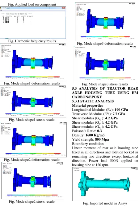
Fig. Imported model in Ansys
Fig. Created mesh on component
Fig. Applied load on component
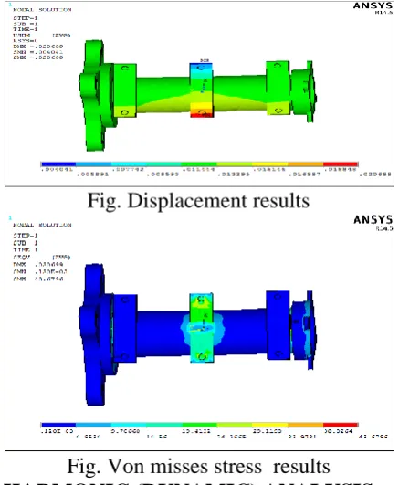
Fig. Displacement results
Fig. Von misses stress results
HARMONIC (DYNAMIC) ANALYSIS Boundary condition
Linear moment of rear axle housing tube fixed in all directions and rotation locked in remaining two directions except horizontal direction. Power load 500N applied on housing tube at 120 rpm.
Fig. Imported model in Ansys
Fig. Applied load on component
Fig. Harmonic frequency results
Fig. Mode shape1 deformation results
Fig. Mode shape1 stress results
Fig. Mode shape2 deformation results
Fig. Mode shape2 stress results
Fig. Mode shape3 deformation results
Fig. Mode shape3 stress results
5.3 ANALYSIS OF TRACTOR REAR AXLE HOUSING TUBE USING HM CARBON/EPOXY
5.3.1 STATIC ANALYSIS Material properties
Longitudinal Modulus (EX): 190 GPa Transverse Modulus (EY): 7.7 GPa
Shear modulus (Gxy ): 4.2 GPa Shear modulus (Gyz ): 4.2 GPa Shear modulus (Gxz ): 4.2 GPa Poisson’s Ratio: 0.3
Density: 1600 Kg/m3
Yield strength: 800 Mpa Boundary condition
Linear moment of rear axle housing tube fixed in all directions and rotation locked in remaining two directions except horizontal direction. Power load 500N applied on housing tube at 120 rpm.
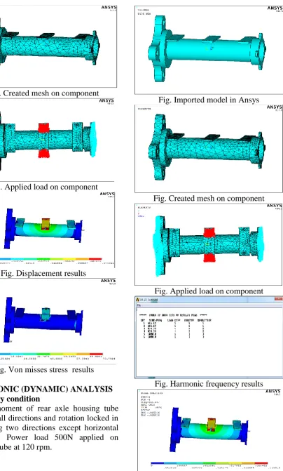
Fig. Created mesh on component
Fig. Applied load on component
Fig. Displacement results
Fig. Von misses stress results
HARMONIC (DYNAMIC) ANALYSIS Boundary condition
Linear moment of rear axle housing tube fixed in all directions and rotation locked in remaining two directions except horizontal direction. Power load 500N applied on housing tube at 120 rpm.
Fig. Imported model in Ansys
Fig. Created mesh on component
Fig. Applied load on component
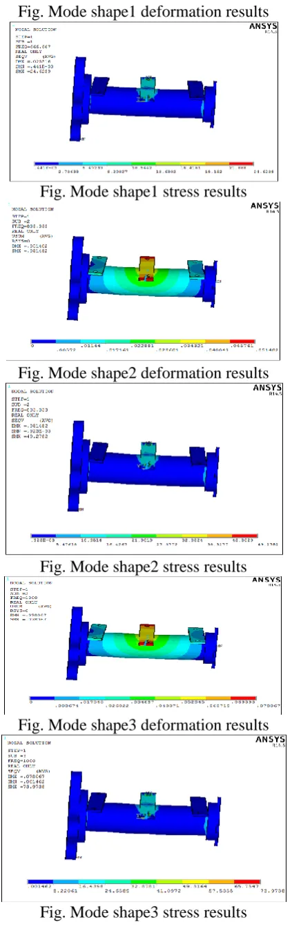
Fig. Mode shape1 deformation results
Fig. Mode shape1 stress results
Fig. Mode shape2 deformation results
Fig. Mode shape2 stress results
Fig. Mode shape3 deformation results
Fig. Mode shape3 stress results
RESULTS AND CONCLUSION
In this project, tractor’s rear axle housing tube was analyzed completely using different materials. Results are given below.
References
[1] Kolator, B. and Białobrzewski, I.,“A simulation model of 2WD tractor
performance,” Compututer and
Electronics in Agriculture, ELSEVIER, Vol. 76, No. 2, 2011, pp. 231-239. [2] Goyal, S. K., Chandra, S. and Chandra,
S.,“A study on fuel consumption and work performance os different tractors with tillage implements,” Society for Recent Development in Agriculture, Vol. 10, No. 2, 2010, pp. 270-274. [3] Chaudhari, P. C., Sonara, V. D. and
Rathod, P. P.,“Analysis and Design of Tractor Rear Axle using Finite Element Method - A review,” Internaltional Journal of Advance Engineeering and Research Development, Vol. 2, Iss. 3, 2015, pp. 105-109.
[4] KISSsoft calculation programs for
machine design.
http://www.kisssoft.com
[5] Nanaware, G. K., and Pable, M. J., "Failure of Rear Axle Shaft of 575 DI Tractors", Engineering Failure Analysis, ELSEVIER, Vol. 10, 2003, pp. 719-724.
[6] Zhijun, W., and Lihua, Z., "Optimal Design for Rear Drive Axle House Based on Fuzzy Reliability Robust Analysis", International Conference on
Chemical, Material and Food
Engineering, 2015, pp. 875–880.
Agricultural Health and Safety: Recent Advances, vol. 4, no. 3, 2009 pp. 303– 307.
[8] Langhart, J., and Bae, I., “How to get Most Realistic Efficiency Calculation for Gearboxes?”, International Gear Conference, ELSEVIER, August 2014, pp. 869-878.
[9] Weis, P., Kučera, Ľ., Pecháč, P., and Močilan, M.,“Modal Analysis of Gearbox Housing with Applied Load,” Procedia Engineering, ELSEVIER, Vol. 192, 2017, pp. 953–958.
[10] Marques, P., Fernandes, C., and Martins, R., “Power loss in a planetary
gearbox”, International Gear