Article
NEURAL CONTROLLER WITH ONLINE
LEARNING ON NONLINEAR SYSTEM IN A
CYLINDRICAL TANK
MAICO CAMERINO 1,* and FILIPE PACHECO 2
1 Senai Cimatec; [email protected] 2 Senai Cimatec; [email protected]
* Correspondence: [email protected]; Tel.: +55-071-9972-88175
Abstract: Most systems that are the subject of control engineering studies have some non-linearity. An example of this is the horizontal cylindrical tank, commonly used in process industries. To deal with cases like this, several control theories have been developed over time, each one presenting better results in certain systems. This work presents an alternative for the control of nonlinear systems, without necessary modeling or previous information about the system, based on a new optimization law for the artificial neural network training in real time.
Keywords: Neural Controller; Nonlinear control; Cylindrical Tank.
1. Introduction
One of the most fundamental characteristics in nonlinear dynamic systems is the disobedience to the principle of superposition, valid only in linear systems. The result of this observation has the consequence that for different references provided to the controller in a non-linear system, it requires control efforts that vary in a non-linear way when compared with the variations of the reference. This explains why linear controllers, such as PID, in some moments has efficient results and another inefficient in different points in non-linear systems [1].
A very recurrent alternative is the development of control theories based on linearization of the process around a usual point of operation. As example, it is possible to mention PID controllers with multiple tuning [2] and controller based on linear model (MPC) [3]. Some alternative linearization techniques have been developed and applied such as Adaptive fuzzy controller [4] neural model based controller (NNMPC) [5], which can have direct and / or indirect models of the system [6], it has being an evolution of the idea presented by Widrow and Walach [ 7 ] in theirs book Adaptive Inverse Control.
In the industry process, the most advanced controls are model-based, MPC [8]. However, this type of controller has some deficiencies in its industrial applications. The majority model-based controllers in industry have linear models of the controlled processes. As the process moves away from the creation point of the model, the efficiency of the controller tends to fall due to the prediction errors attributed to the linear model. Additionally, the periodic non-updating of the models, knowing that, the processes undergo changes in their dynamics with the years of operating time extends.
The alternative found by [5] demonstrates a more robust response, in order to increase the efficiency of this type of controller in non-linear systems. However, this training occurs by batch, offline, and does not contemplate the second problem cited in the previous paragraph. Searching to present an alternative solution to already existing methods, the main idea of this article is to develop a neural controller that could control an unknown system, that is, without models, without previous information, with randomly initiated synaptic weights, and still capable of
adapt to the process changes with real time learning. Thus, a new optimization function is presented to be applied in joint with the Backpropagation algorithm.
2. Experiments
One of the most-known algorithms for training a neural network is the Backpropagation, such algorithm can be used to train a neural controller by batch [9] or in real time [10]. The training algorithm of a neural network is based on the idea of the mean square error (MSE), whose function is defined as:
E =(y − y)
2 (1)
Where the value of ycorresponds to the output of the neural network. This value can be defined
by the following equation:
y = φ(M[X] ) (2)
Which the function φrepresents the activation function of the neuron, M represents the matrix
of synaptic weights that connect the input layer data to their respective neurons, and finally, X
which represents the input vector in this neuron. Assuming that the equation (1) is an optimization
problem and assuming as the matrixMthe decision variables of the problem, it arrives at:
∂E ∂y
∂y ∂φ
∂φ
∂M= (y − y)φ (M[X] )[X] (3)
Writing the equation (3) through the gradient optimization method, it has to:
∆M = −α∂E
∂M (4)
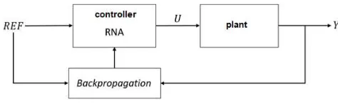
The equations 3 and 4 summarize the Backpropagation algorithm for only one neuron. The type of controller that this article proposes to develop, such an algorithm written in this way, is not compatible with the definition of the problem, which there is not known model of the plant and could learn in real time. Figure 1 shows the block diagram of the control structure as known in the literature.
Figure 1. Block diagram of the neural controller known in the literature.
As is shown above, the output of the network is represented by U and no more for y, therefore
can not be written as equation 1 due the output Y the process that will be compared to the value of
REF is an function of (P), plant,dependent on U, then the equation 1 should be rewritten as:
E =(y − P(U))
2 (5)
The current literature proposes two ways of training a neural network to control systems in this
way. The first way is the development of a dynamic model that represents the plant (P). The
advantages of this method is possibility of real-time training, without the necessary of previous data.
The great disadvantage is the inefficiency of the controller until a suitable model of the plant (P) is
In both cases, it is necessary to acquire data to develop models. To avoid this problem, it was necessary to create a new objective function that the controller could control with the Backpropagation algorithm the system in real time. This equation is demonstrated in the matrix form as:
J =1
2 Q y − y + ψ y − y (U − U ) + R(U − U ) (6)
Where:
U = the current control action
U = previous control action
Q, R e Ψ = variable weighting of the controller (tuning)
Equation 1 should be replaced by equation 6 as an objective function to be applied with control form by the Backpropagation algorithm. The block diagram illustrating the controller in closing the loop feedback of the controller remains the same as that shown in figure 1. Using by this objective function, it is possible to control the process, even if the system changes, as in variant systems in time, which is a great advantage compared to controllers that have static model.
A disadvantage of this approach in comparison to controllers that have a model, even if linearized, is the impossibility of predicting the effect of their control actions that have been implemented or that will be, or even in PID controllers where there is derivative action that seeks to anticipate the correction. As a result of this limitation, in dynamic systems whose system response to the input stimulus needs time to stabilize, the system oscillates until it stabilizes at the desired reference value. Such behavior resembles that of a sub-damped second-order system, as can be seen in the following section.
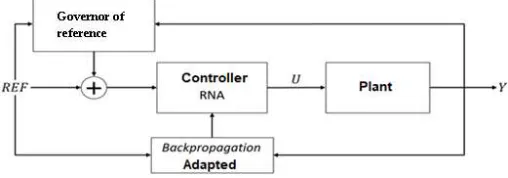
In order to try to accelerate the correction of the system and minimize possible oscillations, this work utilizes the idea of governor of reference. Such implementation is not new in control systems, but remains a great artifice for smoothing corrections in non-linear systems. With this adaptation, the block diagram illustrating the controller presented by this work in figure 1 is changed to the following figure.
Figure 2. Diagram of neural controller blocks with governor of reference.
The function used by the governor of reference is defined as follow:
G = k(∆Y) = k(Y − Y ) (6)
The choice of this function is based on the idea that the rate of change of the plant output in relation to time. When the subtraction result, contained within the parentheses, is greater than zero, it means that the output variable is at elevation, what for a stable system, should mean that the reference is at a value above the controlled variable. For 𝑘 < 0, implies that the governor of
reference should reduce the input value so the controller has a smaller error than the actual one, doing the correction smoother. The inverse occurs when the subtraction results in a negative value.
The system chosen for the application of this controller was a horizontal cylindrical tank. Such system has non-linear characteristics; hence, the volume inside the tank does not change linearly with the variation of height. This system had its analytical modeling described in [11]. Below is the figure that represents the system.
Figure 3. Graphic illustration of horizontal cylindrical tank.
This system has as manipulated variable the incoming flow, while the drainage of water occurs naturally by the action of gravity. Equation 7 represents the dynamics of the system as a function of time, thus allowing numerical simulation of the effects of control actions implemented by the neural controller as well as a PID controller used to compare the results of the controller developed by this work.
dh
dt =
1
2r 2hr − h²
r²
F (t) − C C gh(t)
L (7)
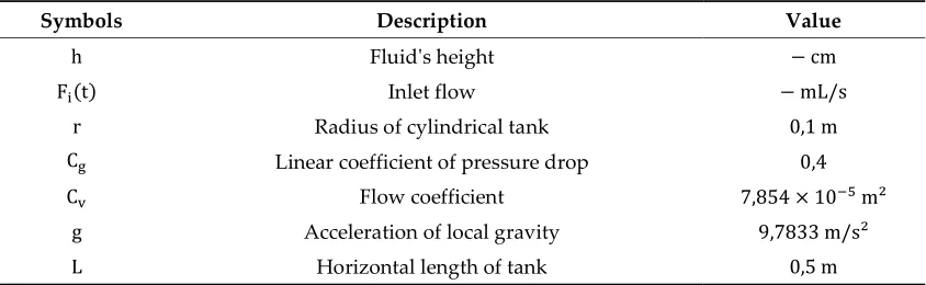
Table 1. Descriptions of checks and variables.
Symbols Description Value
h Fluid's height − cm
F (t) Inlet flow − mL/s
r Radius of cylindrical tank 0,1 m
C Linear coefficient of pressure drop 0,4
C Flow coefficient 7,854 × 10 m²
g Acceleration of local gravity 9,7833 m/s²
L Horizontal length of tank 0,5 m
Figure 4. System response with PID controller.
It is possible to note that for large changes in the reference, this linear controller suffers with overshoots in its control action. It is also notable that in some moments with great variations its control action gets to be zeroed, which causes greater oscillation due to the value that is accumulated in the integrative action of the algorithm.
Figure 5 represents the response of the system to the neural controller without the anticipatory action of the governor of reference. It is observed that it takes a long time for the system to stabilize, even though the control action is always close to the steady state value.
Figure 5. System response with Neural controller without governor of reference.
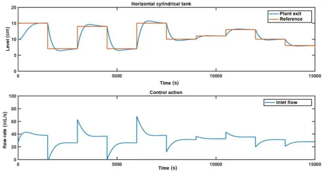
Figure 6. System response with Neural controller with governor of reference.
The control amplitudes are also shown to be smaller. All smoothness that can only be achieved due to the action of the reference controller since the neural controller with real-time learning has no action that can anticipate its correction. Figure 7 represents the reference desired for the blue level and in red the reference that is presented to the controller after the action of the reference controller acting according to equation (6).
Figure 7. Governor of reference’s Action.
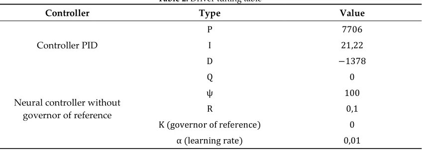
Table 2 shows the values used to tune the controllers in the simulations. The tuning of the PID controller was accomplished by Auto Tune Matlab tool, while others were set by trial and error.
Table 2. Driver tuning table
Controller Type Value
Controller PID
P 7706
I 21,22
D −1378
Neural controller without governor of reference
Q 0
ψ 100
R 0,1
K (governor of reference) 0
Neural controller with governor of reference
Q 0
ψ 100
R 0,1
K (governor of reference) −100
α (learning rate) 0,2
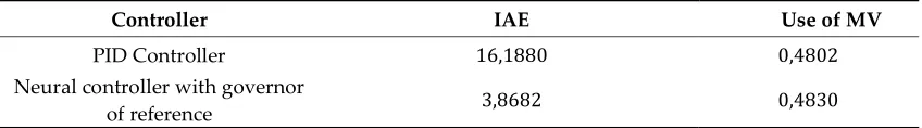
In table 3 is listed the two parameters for comparison of performance of both controllers. In the first parameter is the IAE, integral absolute error, while the second represents the sum of the use of the MV throughout the simulation. The data are self-explicative. It is notable that the use of the governor of reference in assisting the neural controller greatly accelerates its correction with the use of practically the same amount of MV.
Table 3. Driver performance
Controller IAE Use of MV
PID Controller 16,1880 0,4802
Neural controller with governor
of reference 3,8682 0,4830
4. Conclusions
At the end of the analysis of the results, it is possible to infer that the use of the neural controller has advantages in its performance against the linear controller in non-linear systems. However, the proposed controller performed very slowly in its correction, given that it has no way to anticipate its correction, as does the derivative action in PID controller. Thus, it was necessary to use an artifice known as governor of Reference, which realizes part of the work that would be done by the controller is previously performed by the governor, in order to the controller can reproduce a smoother control effort. The next steps in the search line for this type of controller is to analyze its performance on time-variant systems, when there is a real need for flexible parameters for system controllers like this.
References
1. ÅSTRÖM, K.J.; HÄGGLUND, T. Revisting the Ziegler-Nichols step response method for PID control. Journal of Process Control, v. 14, n. 6, p. 635 – 650 – 2004.
2. NANDONG, J. A multi-scale Control Approach for a PID Controller Tuning based on Complex Models. CHEMECA. Australia, 2014.
3. COSTA, ERBERT A.; PATARO, IGOR M.; PACHECO, FILIPE S.; MARTINS, ANDRÉ A. F..Controladores Preditivo com Estabilidade Garantida em duas Camadas para Sistemas com Polos Integradores Repetidos. CBA – 2018.
4. KHOOBAN, M. H.; NIKNAM, T.. A new intelligent online Fuzzy tuning approach for multi-area load frequency control: Self adaptive Modified Bat Algorithm. Elsevier – Eletrical Power and Energy Systems. v. 71, p. 254 – 261 – 2015.
5. NARIMANI, M.; WU, B.; YARAMASU, V.; CHENG, Z.; ZARGARI, N. R. Finite Control-Set Model-Predective Control (FCS-MPC) of Neasted Neural Point-Clamped (NNPC) Converter. IEEE Transactions on Power Electronics, v. 30, n. 12, 2015.
6. KAMALASADAN, S.; GHANDAKLY, A.A.. A neural network based intelligent model reference adaptive controller. IEEE International conference on Computational Intelliegence for Measurement Systems and Applications, 2004.
7. WIDROW, B.; WALACH, E.. Adaptive Inverse Control. Prentice Hall – New Jersey – 1996.
9. HEERTJES, M., TSO, T.. Robustness, convergence, and Lyapunov Stability of a nonlinear iterative learning control applied at a Wafer Scanner. American Control Conference, 2007.
10. ZHANG, Y., SEN, P., HEARN, G.. An on-line trained adaptative neural controller. IEEE Control Systems, v, 15, n, 5, 1995.