Profiled SCA with a New Twist:
Semi-supervised Learning
Stjepan Picek1, Annelie Heuser2, Alan Jovic3, Axel Legay4, and Karlo Knezevic3
1
Delft University of Technology, The Netherlands
2 CNRS, IRISA, Rennes, France
3
University of Zagreb, Croatia
4
Inria, IRISA, Rennes, France
Abstract. Profiled side-channel attacks represent the most powerful category of side-channel attacks. In this context, the attacker gains ac-cess of a profiling device to build a precise model which is used to attack another device in the attacking phase. Mostly, it is assumed that the attacker has unlimited capabilities in the profiling phase, whereas the attacking phase is very restricted. We step away from this assumption and consider an attacker who is restricted in the profiling phase, while the attacking phase is less limited as in the traditional view. Clearly, in general, the attacker is not hindered to exchange any available knowledge between the profiling and attacking phase. Accordingly, we propose the concept of semi-supervised learning to side-channel analysis, in which the attacker uses the small amount of labeled measurements from the profil-ing phase as well as the unlabeled measurements from the attackprofil-ing phase to build a more reliable model. Our results show that semi-supervised learning is beneficial in many scenarios and of particular interest when using template attack and its pooled version as side-channel attack tech-niques. Besides stating our results in varying scenarios, we discuss more general conclusions on semi-supervised learning for SCA that should help to transfer our observations to other settings in SCA.
1
Introduction
Side-channel analysis (SCA) consists of extracting secret data from (noisy) mea-surements. As of today, it is made up of a collection of miscellaneous techniques, combined in order to maximize the probability of success, for a low number of trace measurements and as low computation complexity as possible.
(ML) techniques. When working with the typical assumption for profiled SCA that the profiling phase is not bounded, the situation actually becomes rather simple if neglecting computational costs. If the attacker is able to acquire an unlimited amount of traces, the template attack (TA) is proven to be optimal from an information theoretic point of view (see e.g., [1, 2]). In that context of unbounded and unrestricted profiling phase, ML techniques seem not to be needed.
Stepping away from the assumption on unbounded number of traces the situ-ation becomes much more interesting and of practical relevance. A number of re-sults in recent years showed that in those cases, machine learning techniques can actually significantly outperform template attack (see e.g., [3]). Recently, these results were further strengthened when showing that deep learning techniques can outperform both template attack and machine learning techniques [4, 5].
Still, all of the aforesaid attacks work under the assumption that the attacker has a (significantly) large amount of traces to learn the model. The opposite case would be to learn a model without any labeled examples. Machine learning approaches (mostly based on clustering) have been proposed up to now only for public key encryption schemes where only two possible classes are present – 0 and 1 – and where the key is guessed using only a single-trace (see e.g., [6]). In the case of differential attacks (using more than one encryptions) and using more than two classes, to the best of our knowledge unsupervised machine learning techniques have not been studied yet.
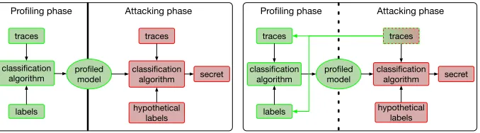
In this paper, we aim to address a scenario lying between supervised and unsupervised learning, the so-called semi-supervised learning in the context of SCA. Figure 1 illustrates the different approaches of supervised (on the left) and semi-supervised learning (on the right). Supervised learning assumes that the attacker first possesses a device similar to the one under attack. Having this additional device, he is then able to build a precise profiling model using a set of measurement traces and knowing the plaintext/ciphertext and the secret key of this device. In the second step, the attacker uses the beforehand profiling model to reveal the secret key of the device under attack. For this, he additionally measures a new set of traces, but as the key is secret he has no further information about the intermediate processed data and thus build hypotheses. Accordingly, the only information which the attacker transfers between the profiling phase and the attacking phase is the profiling model he builds.
traces
labels classification
algorithm profiled model
traces
hypothetical labels classification
algorithm secret Profiling phase Attacking phase
traces
labels classification
algorithm profiled model
traces
hypothetical labels classification
algorithm secret traces
Profiling phase Attacking phase
Fig. 1: Profiling side-channel scenario: traditional (left), semi-supervised (right)
traces is (very) low, and thus any additional data is helpful to improve the model estimation.
From a practical perspective, the assumption of a bounded (restricted) pro-filing phase is more reasonable due to resource constraints (e.g., time, space, computational power, man power) for hardware security evaluators and actual attackers. When considering possible restrictions for attackers, one example that naturally comes in mind is the “lunchtime” attack. There, the attacker is only able to gain access of the profiling device, on which he has (or a group of persons have) full knowledge of the properties, during the lunch time. Accordingly, the profiling phase is extremely limited in the number of traces. On the contrary, for the device under attack any similar device is suitable so the attacker is able to gain a larger amount of traces for the key recovery.
To show the efficiency and applicability of semi-supervised learning for SCA, we conduct extensive experiments where semi-supervised learning is outperform-ing supervised learnoutperform-ing if certain assumptions are satisfied. More precisely, the results show a number of scenarios where the accuracy on the test set is signif-icantly higher if semi-supervised learning is used (when compared to the “clas-sical” supervised approach). We start with the scenario we call the “extreme profiling” where the attacker has only a very limited number of traces to learn the model. From there, we increase the number of available traces making the attacker more powerful until we reach a setting where there is no more need for the semi-supervised learning. Still, our results show that using semi-supervised learning even in those contexts, is not deteriorating the efficiency of attacks.
direction we take in this paper. Also our analysis is not restricted to only one labeled class in the learning phase.
Note, even if the basic principle to combine labeled and unlabeled data is well-known in the area of machine learning, we want to stress that it is not restricted to the machine learning algorithms. Summarizing, our main contributions are:
1. We introduce a new perspective on profiled side-channel analysis called semi-supervised learning, where the setting we use is justified from the theoretical perspective.
2. We conduct extensive experiments in order to assess the efficiency of semi-supervised learning. Our experiments vary with the respect to the level of noise, number of classes, number of traces, semi-supervised learning paradigms, and classification algorithms.
3. We analyze the benefits and limits of applicability of semi-supervised learn-ing in side-channel analysis and give recommendations when to use it. 4. We show that semi-supervised learning can be used to stabilize covariance
matrices for template attack.
We emphasize that we primarily focus on improving the accuracy if the profiling phase is limited. Since we are considering extremely difficult scenarios, the im-provements one can realistically expect are often not too big (i.e., in the range of only a few percent). Still, we consider any improvement to be relevant since it makes the attack easier, while not requiring any additionally knowledge or measurements.
The rest of this paper is organized as following. In Section 2 we discuss the semi-supervised paradigm, how can it be used in order to boost classification results, and the classes of algorithms we consider. Next, in Section 3 we give de-tails about the datasets we consider, the algorithms we use, and our experimental evaluation procedure. Section 4 presents the experimental results for both semi-supervised experiments as well as for the semi-supervised experiments, which serve as a baseline case. Section 5 brings discussion about results obtained, pitfalls one can face when using semi-supervised learning, and possible future research directions. Finally, Section 6 offers a brief conclusion.
2
Semi-supervised Learning
mea-surements. The attacking device is another device on which he tries to reveal the secret key using as less encryptions (and thus side-channel measurements) as possible.
In unsupervised learning, one has at his disposal a number of test examples consisting only of measurements (there is no information about the correspond-ing classes). Then, on the basis of those measurements one tries to find some structure in the data. This scenario maps to an attacker who has access to only one device with unknown properties. On this device he tries to reveal the secret key using as less encryptions as possible.
Semi-supervised learning (SSL) is positioned in the middle between super-vised and unsupersuper-vised leaning. There, the basic idea is to take advantage of a large quantity of unlabeled data during a supervised learning procedure [8]. This approach assumes that the attacker is able to possess a device to conduct a profiling phase but does not have unlimited capacities. This may reflect a more realistic scenario in some practical applications, as the attacker may be limited by time, resources, and also face implemented countermeasures which prevent him from taking an unlimited amount of side-channel measurements while knowing the secret key of the device.
In the following, we describe semi-supervised learning in a more formal way and discuss why it may (or may not) work. Afterwards we discuss two differ-ent approach used for semi-supervised learning in this paper and describe their implementations. We note that we use interchangeably the notions of training, profiling, and learning phase as well as testing or attacking phase.
2.1 Notation and Types of Semi-supervised Learning
Letx= (x1, . . . , xn) be a set ofnsamples where each samplexiis assumed to be drawn i.i.d. from a common distributionX with probabilityP(x). This setxcan be divided into three parts: the points xl= (x1, . . . , xl) for which we know the labelsyl= (y1, . . . , yl) and the pointsxu= (xl+1, . . . , xl+u) for which we do not know the labels. Additionally, the third part is the test setxt= (xl+u+1, . . . , xn) for which labels are also not known. We see that differing from the supervised case where we also do not know labels in the test phase, here unknown labels appear already in the training phase. As for supervised learning, the goal of semi-supervised learning is to predict a class for each sample in the test set xt= (xl+u+1, . . . , xn). For semi-supervised learning two learning paradigms can be discussed: transductive and inductive learning [9]. In transductive learning (which is a natural setting for some semi-supervised algorithms), predictions are performed only for the unlabeled data on a known test set. The goal is to opti-mize the classification performance on the test set. More formally, the algorithm makes predictionsyt= (yl+u+1, . . . , yn) onxt= (xl+u+1, . . . , xn). In inductive learning, the goal is to find a prediction function defined on the complete space
states when solving a problem, one should not try to solve more difficult prob-lem as an intermediate step. From the algorithm class perspective, we will use two approaches in order to achieve successful semi-supervised learning, namely: self-training [9] (Section 2.3) and graph-based algorithms [9, 10](Section 2.4).
2.2 Why Semi-supervised Learning (Does Not) Work
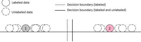
In Figure 2 we show how semi-supervised learning can help in the process of classification. It depicts a binary classification problem (two classes) for which some samples are labeled while others do not have labels. Assuming that each class makes a coherent group, we observe that the decision boundary between classes changes when also using unlabeled data when compared to the scenario when only labeled data is used.
Fig. 2: Classification with semi-supervised learning.
Although on an intuitive level semi-supervised learning sounds as an ex-tremely powerful paradigm (after all, humans learn through semi-supervised learning) the results show that is not always the case. More precisely, when comparing semi-supervised learning with supervised learning, it is not always possible to obtain more accurate predictions. Consequently, here we are inter-ested in cases where semi-supervised learning can outperform supervised learn-ing. In order to be able to do so, the following needs to hold: the knowledge on p(x) one gains through unlabeled data has to carry useful information for inference ofp(y|x). In the case this is not true, semi-supervised learning will not be better than supervised learning and can be even worse. To assume a struc-ture about the underlying distribution of data and to have useful information in the process of inference, we use two main assumptions which should hold when conducting semi-supervised learning [9]. We first argue why these assumption are likely to hold for SCA and further use simulated data (see Section 2.4) for illustration.
andy2. Intuitively, this assumption tells us that if two samples (measurements) belong to the same cluster, then their labels (e.g., their Hamming weight or in-termediate value) should be close. Note that, this assumption also implies that, if two points are separated by a low-density region, then their labels need not be close. The smoothness assumption should generally hold for SCA, as the power consumption (or electromagnetic emanation) is related to the activity of the device. For example, a low Hamming weight or low intermediate value should result in a low side-channel measurement.
Manifold Assumption The high-dimensional data lie on or close to a low-dimensional manifold. If the data really lie on a low-low-dimensional manifold, then the classifier can operate in a space of the corresponding (low) dimension. In-tuitively, the manifold assumption tells us that a set of samples is connected in some way: e.g., all measurements in the Hamming weight class 4 lie on their own manifold, while all measurements for the Hamming weight class 5 lie on a different but nearby manifold. Then, we can try to develop representations for each of these manifolds using just the unlabeled data while assuming that the different manifolds will be represented using different learned features of the data.
2.3 Self-training
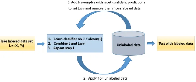
In self-training (or self-learning), any classification method is selected and the classifier is trained with the labeled data. Afterwards, the classifier is used to classify the unlabeled data. From the obtained predictions, one selects only those instances with the highest output probabilities (i.e., where the output probability is higher than a given thresholdσ) and then adds them to the labeled data. This procedure is repeated k times. A depiction of this process is given in Figure 3. Self-training is a well-known semi-supervised technique and one that is probably the simplest to start with [9]. The biggest drawback with this technique is that it depends on the choice of the underlying classifier and that possible mistakes re-inforce themselves as the number of repeats increase. Naturally, one expects that the first step of self-learning will introduce errors (wrongly predicted classes). It is therefore important to retain only those instances for which the prediction probability of the class is high. Note that a very high class prediction probabil-ity (even 100%) does not guarantee that the actual class is correctly predicted. The assumption taken by the self-training algorithm is the same as the assump-tion taken for the underlying supervised learner – i.e., when we use SVM as the classifier, then we work with the manifold assumption while if we use Naive Bayes then we use the semi-supervised smoothness assumption (alongside the independence assumption, which is a standard for Naive Bayes).
Fig. 3: Depiction of self-training process.
unlabeled set is optimized. To speed up the cross-validation process we imple-mented a parallel program in Java programming language. We concurrently train classifier models, choosing one with the best threshold value.
Except parallel cross-validation, we implement a custom Java wrapper around Weka [11] in order to better fulfill our requirements. To speed up the labeling process of the unlabeled samples, we use a parallel stream filter. The stream filter selects the samples with class probability higher than the threshold and classifies them into appropriate classes. We repeat the labeling process as long as the classification accuracy on the testing set is growing or if samples exist where the output probability of the classifier is higher than the threshold. The second readjustment is important because we noticed that even a wrong labeling could improve the classifier generalization on the testing set. Here, by classifier generalization we consider how well will the classifier behave on a yet unseen dataset.
2.4 Graph-based Learning
In graph-based learning, the data are represented as nodes in graphs where a node is both labeled and unlabeled example. The edges are labeled with the pairwise distance of incident nodes and if an edge is not labeled, it corresponds to the infinite distance. Most of the graph-based learning techniques depend on the manifold assumption. Most of the graph-based learning methods refer to the graph by utilizing the graph Laplacian. Let G= (E, V) be a graph with edge weights given by w:E →R. The weight w(e) of an edgee corresponds to the
similarity of the incident nodes and a missing edge means no similarity. The similarity matrixW of graph Gis defined as:
Wij = (
w(e) ife= (i, j)∈E
0 ife= (i, j)∈/E (1)
– normalized graph LaplacianL=I−D−1/2W D−1/2,
– unnormalized graph LaplacianL=D−W.
In our experiments, we use graph-based learning technique called Label spreading that is based on normalized graph Laplacian. As a classifier within the Label spreading, we usek-nearest neighbors (k-NN) (i.e., the technique how to assign labels) since it produces sparse matrix that can be calculated very quickly. k-nearest neighbors is the basic non-parametric instance-based learn-ing method. The classifier has no trainlearn-ing phase; it just stores the trainlearn-ing set samples. In the test phase, the classifier assigns a class to an instance by de-termining the k instances that are the closest to it, with respect to Euclidean distance metric: d(xi, xj) =pP
n
r=1(ar(xi)−ar(xj))2. Here, ar is the r-th at-tribute of an instance x. Class is assigned as the most commonly occurring one among the k-nearest neighbors of the test instance. This procedure is repeated for all test set instances. The simple method is highly useful and accurate in practice, especially in the cases when there are many more instances than the number of attributes and in the presence of noise (fork¿1) [12]. The method is encumbered with the problem of irrelevant attributes - as all of them are used in determining the distance, some irrelevant attributes may contribute to false de-cisions. Although feature selection (and dimensionality reduction) methods may be used to eliminate the majority of irrelevant attributes fork-NN, this usually slows the whole procedure and is not examined in detail in this work [13].
We use Label spreading as implemented in Python [14] but we wrote a custom wrapper around it in order to better suit our requirements. There, instead of using all measurements obtained from semi-supervised learning, we use only those samples that have the highest classification probabilities (similar to self-training).
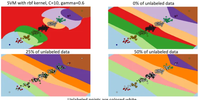
Fig. 4: Decision boundaries after SVM with only labeled data and semi-supervised learning using 0%, 25%, 50% of unlabeled data. 0% means there is no semi-supervised learning phase since all data is known. For 25%, 50% labels are predicted using label spreading.
Finally, we note that both transductive and inductive learning are used in this paper. With self-training in each step we build a model, which is the example of inductive learning (although we use only the last obtained model on test data). With Label spreading we first use transductive learning to find the labels for the unlabeled traces in the training set. Then, we use inductive learning to find the model to be used on test set.
3
Experimental Setting
3.1 Classification algorithms
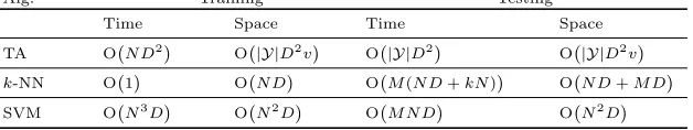
The techniques described next are used as classification algorithms in semi-supervised and semi-supervised settings. Note that the same technique can be used in both phases. We display in Table 1 the time and space complexities for classifi-cation algorithms we use and give details on algorithms in subsequent sections. In Table 1, N is the number of samples in the training set,M is the number of samples in the test set,D is the number of attributes, and|Y|is the number of classes of the target attribute.
Template Attack The template attack (TA) relies on the Bayes theorem such that the posterior probability of each class valuey, given the vector ofNobserved attribute valuesx:
p(Y =y|X =x) = p(Y =y)p(X =x|Y =y)
Table 1: Time and space complexities
Alg. Training Testing
Time Space Time Space
TA O N D2 O
|Y|D2v O
|Y|D2 O
|Y|D2v
k-NN O 1
O N D
O M(N D+kN)
O N D+M D
SVM O N3D
O N2D
O M N D
O N2D
whereX =xrepresents the event thatX1=x1∧X2=x2∧. . .∧XN =xN. When used as a classifier, p(X = x) in Eq. (2) can be dropped as it does not depend on the class y. Accordingly, the attacker estimates in the profiling phasep(Y =y) andp(X =x|Y =y) which are used in the attacking phase to predict p(Y = y|X =x). Note that the class variable Y is discrete while the measurementX is continuous. So, the discrete probabilityp(Y =y) is equal to its sample frequency wherep(Xi=xi|Y =y) displays a density function.
Mostly in the state of the art, TA is based on a multivariate normal distri-bution of the noise and thus the probability density function used to compute p(X =x|Y =y) equals:
p(X =x|Y =y) = p 1 (2π)D|Σ
y|
e−12(x−µy) TΣ−1
y (x−µy), (3)
whereµyis the mean overXfor 1, . . . , DandΣythe covariance matrix for each classy. The authors of [15] propose to use only one pooled covariance matrix to cope with statistical difficulties that result into low efficiency. We will use both version of the template attack, where we denote pooled TA attack asT Ap.
Naive Bayes The Naive Bayes classifier [16] is also based on the Bayesian rule, but is labeled “Naive” as it works under a simplifying assumption that the pre-dictor features (measurements) are mutually independent among theDfeatures, given the class value. Existence of highly-correlated features in a dataset can thus influence the learning process and reduce the number of successful predictions. Additionally, Naive Bayes assumes normal distribution for predictor features. As the classifier assumes independence amongD, individual probabilities can be multiplied in Eq. (2):
p(X=x|Y =y) = D Y
i=1
p(Xi=xi|Y =y). (4)
Naive Bayes classifies as:
p(Y =y|X=x) =p(Y =y) D Y
i=1
As we assume a univariate normal distribution, the probability density function used to computep(Xi=xi|Y =y) equals:
p(Xi=xi|Y =y) = 1 p
2πσy e−
(xi−µy)2
2σ2y . (6)
Support Vector Machines Support Vector Machine (SVM) is a kernel based machine learning technique used to accurately classify both linearly separable and linearly inseparable data [17]. The SVM algorithm is parametric and deter-ministic. The basic idea when the data are not linearly separable is to transform them to a higher dimensional space by using a transformation kernel function. In this new space, the samples can usually be classified with a higher accuracy. Many types of kernel functions have been developed, with the most used ones being polynomial and radial-based. As a learning method, a Sequential Minimal Optimization (SMO) algorithm is used [18, 19]. Since SMO is a binary classifi-cation algorithm, for multiclass classificlassifi-cation purposes it is adapted to perform n×(n−1)/2 binary classifications. In SVM with radial kernel, a low cost of the margin parameterCmakes the decision surface smooth, while a highCaims at classifying all training examples correctly. The radial kernel parameterγdefines how much influence a single training example has, where the larger γ is, the closer other examples must be to be affected. The radial kernel is considered to be a good choice when there is no expert knowledge about the problem and the number of features is not too high and when there is no linear separation between the data [20].
3.2 Evaluation criteria
We use the following measures to depict our results. Our main measure is the ac-curacy, which is the percentage of correctly classified instances:ACC= T PT P+T N. In the training phase for supervised approaches as well as in the training phase for semi-supervised learning we use only accuracy as a measure of quality. In the testing phase (and only for ML algorithms), we also report the area under the ROC curve (AUC). The area under the ROC curve is used to measure the accuracy and ROC curve is the ratio between true positive rate and false positive rate. A truly useless test has an area of 0.5, while a perfect test has an area of 1. Values close to 0.5 should be considered similar to a random guess [21]. Usually AUC is used in a comparative way between various methods and there is no absolute value where one can say that all values above it are good.
3.3 Datasets
the number of scenarios would become quite large. Accordingly, we select 50 points of interests with the highest correlation between the class value and data set for all analyzed data sets.
Calligraphic letters (e.g.,X) denote sets, capital letters (e.g.,X) denote ran-dom variables taking values in these sets, and the corresponding lowercase letters (e.g., x) denote their realizations. Letk∗ be the fixed secret cryptographic key (byte) and the random variableTthe plaintext or ciphertext of the cryptographic algorithm which is uniformly chosen. The measured leakage is denoted asX and we are particularly interested in multivariate leakage X =X1, . . . , XD, where D is the number of time samples or features (attributes) in machine learning terminology.
Considering a powerful attacker who has a device with knowledge about the secret key implemented, a set ofN profiling tracesX1, . . . ,XN is used in order to estimate the leakage model beforehand. Note that this set is multi-dimensional (i.e., it has dimension equal to D×N). In the attack phase the attacker then measures additional traces X1, . . . ,XQ from the device under attack in order to break the unknown secret keyk∗.
DPAcontest v2 [22]. DPAcontest v2 provides measurements of an AES hard-ware implementation. Previous works showed that the most suitable leakage model (when attacking the last round of an unprotected hardware implementa-tion) is the register writing in the last round, i.e.,
Y(k∗) = Sbox−1[Cb1⊕k
∗]
| {z }
previous register value
⊕ Cb2
|{z} ciphertext byte
, (7)
where Cb1 and Cb2 are two ciphertext bytes, and the relation between b1 and
b2 is given through the inverse ShiftRows operation of AES. In particular, we choose b1 = 12 resulting in b2 = 8 as it is one of the easiest bytes to attack5. In Eq. (7) Y(k∗) consists in 256 values, as an additional model we applied the Hamming weight (HW) on this value resulting in 9 classes. These measurements are relatively noisy and the resulting model-based signal-to-noise ratio SN R=
var(signal) var(noise) =
var(y(t,k∗))
var(x−y(t,k∗)), lies between 0.0069 and 0.0096.
DPAcontest v4 [23]. The 4th version provides measurements of a masked AES software implementation. However, as the mask is known, one can easily turn it into an unprotected scenario. Though, as it is a software implementation, the most leaking operation is not the register writing, but the processing of the S-box operation and we attack the first round. Accordingly, the leakage model changes to
Y(k∗) =Sbox[Pb1⊕k
∗]⊕ M |{z} known mask
, (8)
where Pb1 is a plaintext byte and we choose b1 = 1. Again we consider the
scenario of 256 classes and 9 classes (considering HW(Y(k∗))). Compared to
5
the measurements from the version 2, the model-based SNR is much higher and lies between 0.1188 and 5.8577.
3.4 Dataset Preparation
In all experiments, we use a set of randomly selected 20 000 measurements (pro-filed traces) from DPAcontest v2 and DPAcontest v4 datasets, with 256 or 9 HW classes (see Section 3.3). These measurements are divided into 2:1 ratio for training and testing sets (i.e., 13 000 in total for training with or without semi-supervised learning and 7 000 for testing). When using semi-supervised learning, the training datasets are divided into 10 stratified folds and evaluated by 10-fold cross-validation procedure.
When considering semi-supervised learning, we divide the training dataset into a labeled set of size l and unlabeled set ofu. Besides the number of traces belonging to labeled and unlabeled sets, we give the percentage shares for both sets.
– (100+12.9k):l= 100 ,u= 12 900 – 0.77% vs 99.23%
– (250+12.75k):l= 250 ,u= 12 750 – 1.93% vs 98.07%
– (500+12.5k):l= 500 ,u= 12 500 – 3.85% vs 96.15%
– (1k+12k):l= 1 000 ,u= 12 000 – 7.69% vs 92.31%
– (3k+10k):l= 3 000 ,u= 10 000 – 23.08% vs 76.92%
– (5k+8k):l= 5 000 ,u= 8 000 – 38.46% vs 61.54%
– (7k+6k):l= 7 000 ,u= 6 000 – 53.85% vs 46.15%
– (10k+3k):l= 10 000 ,u= 3 000 – 76.92% vs 23.08%
4
Experimental Results
In supervised learning, the classifiers are built on labeled sets and estimated on unlabeled sets. We give results here only for the results obtained from the testing phase. When discussing semi-supervised learning, we first learn the classifiers on labeled sets. Then, we learn with the labeled set and unlabeled set in a number of steps where in the each step we augment the labeled set with the most confident predictions from the unlabeled set. Once we cannot add any more measurements, we finish the learning phase. Finally, we conduct the estimation phase on different unlabeled set.
For machine learning techniques that have parameters to be tuned, we con-ducted a tuning phase on labeled sets and use such tuned parameters in conse-quent experimental phases. For SVM with radial kernel, we use C equal to 10 and γ equal to 0.6. When using k-NN with Label spreading, we select k to be equal to 7. Naive Bayes and Template attack do not have parameters to tune.
4.1 Supervised Learning Results
when comparing with semi-supervised learning. Using only 100 traces in profiling phase can be considered as the worst case scenario while using all 13 000 in the profiling phase can be considered as the best case scenario. We can expect that all semi-supervised learning results should be within those ranges (possibly with some small deviations). Indeed, when having extremely small number of traces in profiling phase, it is a natural assumption that adding more measurements in semi-supervised phase should help. Since we must assume there will be at least some portion of measurements incorrectly classified during the semi-supervised learning, we cannot expect semi-supervised learning to be more successful than supervised learning with all traces.
In Table 2 we give results for DPAcontest v4 and we can see that for both 9 and 256 classes, machine learning techniques work well. SVM performs better than Naive Bayes but that is as expected since SVM is more powerful classifica-tion technique. When considering template attacks, we see that pooled version is better since it does not have the problem with covariance matrices instability. As it can be seen, for 13 000 measurements and 9 classes TA and TA pooled perform similarly, which is a strong indication that the covariance matrices got stable and that if there would be further increase in the number of measure-ments, TA may outperform the pooled version. As particularly interesting we consider the efficiency of ML techniques even in scenarios with only 100 to 500 measurements. This leads us to the conclusion that ML is extremely powerful option to be used even in the most extreme profiling cases provided that the level of noise is not too high. Finally, considering the AUC measure we see that the results for ML technique are reliable. The only exceptions are scenarios with 100 and 250 measurements for 256 classes and Naive Bayes classifier where we can see the behavior of the classifier is much more random.
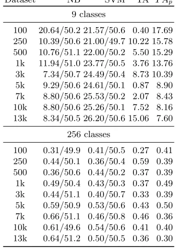
For DPAcontest v2 (Table 3) we see the results are much worse, which is ex-pected due to the higher amount of noise. For the Hamming weight scenario, we can also notice an interesting behavior for the smaller numbers of measurements, e.g., up to 1 000 measurements with Naive Bayes and TA techniques. We see that the accuracies are actually higher than for the cases with more measurements. Although this may look counterintuitive, a closer analysis of results reveals the cause for such a behavior. Since there are very limited number of traces in the profiling phase, some of the classes do not have any correctly trained represen-tatives. As an example, for the scenario with 100 measurements we actually see there are no instances of HW 0, HW 1, HW 7, and HW 8 classes present in the profiling phase. Consequently, the classifiers do not work anymore with 9 classes, but only with 5 classes, which makes it a much simpler classification problem. Naturally, although such results look good, they are not very helpful in the SCA context to reveal the secret key.
Table 2: Testing results, supervised learning, DPAcontest v4, (ACC/AUC)
Dataset NB SVM TA T Ap
9 classes
100 61.51/87.7 69.07/89.8 0.30 45.41
250 64.31/89.3 78.44/93.9 0.30 52.99
500 65.93/90.8 82.70/95.6 0.34 68.93
1k 64.81/91.1 86.56/96.7 1.33 73.14
3k 67.20/91.7 90.81/97.7 5.23 74.86
5k 67.86/91.8 92.00/98.0 2.83 75.79
7k 67.96/91.8 92.84/98.2 11.16 76.51
10k 68.09/91.9 93.26/98.3 0.39 77.24
13k 68.36/91.9 93.71/98.5 75.31 77.74
256 classes
100 1.49/51.5 5.07/60.8 0.30 0.41
250 2.21/54.8 6.77/73.6 0.30 3.32
500 4.89/63.7 10.29/82.5 0.43 6.42
1k 10.46/79.3 13.64/89.1 0.43 10.15
3k 16.49/91.6 22.37/95.0 0.11 16.26
5k 18.04/93.0 27.44/96.5 0.19 19.23
7k 19.46/93.6 30.03/97.2 0.31 20.62
10k 20.14/94.2 33.31/97.8 0.04 22.48
13k 20.17/94.5 34.89/98.1 0.06 23.69
4.2 Semi-supervised Learning Results
In this section, we present the results for semi-supervised learning with self-training (Tables 5 and 7) and for Label spreading (Tables 6 and 8). For all tables we follow the same procedure: we label the unlabeled set in the profiling phase with either self-training or Label spreading. Then, on such labeled sets we use ML and TA classifiers to conduct the testing phase. The results for the testing phase are reported in tables. Recall that self-training is done with two classifiers – Naive Bayes and SVM. We use the same classifier then in semi-supervised phase as in the semi-supervised phase (although that is not a must but simply our decision in order to limit the number of experiments). For template and pooled template attack we use only one of those two models where we select the better performing one.
Table 3: Testing results, supervised learning, DPAcontest v2, (ACC/AUC)
Dataset NB SVM TA T Ap
9 classes
100 20.64/50.2 21.57/50.6 0.40 17.69
250 10.39/50.6 21.00/49.7 10.22 15.78
500 10.76/51.1 22.00/50.2 5.50 15.29
1k 11.94/51.0 23.77/50.5 3.76 13.76
3k 7.34/50.7 24.49/50.4 8.73 10.39
5k 9.29/50.6 24.61/50.1 0.87 8.90
7k 8.80/50.6 25.53/50.2 2.07 8.43
10k 8.80/50.6 25.26/50.1 7.52 8.16
13k 8.34/50.5 26.20/50.6 15.06 7.60
256 classes
100 0.31/49.9 0.41/50.5 0.27 0.41
250 0.44/50.1 0.36/50.4 0.59 0.39
500 0.36/50.6 0.44/50.2 0.37 0.39
1k 0.49/50.4 0.43/50.3 0.37 0.49
3k 0.44/51.1 0.40/50.7 0.33 0.39
5k 0.59/50.9 0.53/50.6 0.43 0.50
7k 0.66/51.1 0.46/50.8 0.46 0.36
10k 0.61/49.6 0.54/50.6 0.41 0.40
13k 0.64/51.2 0.50/50.5 0.36 0.30
have the highest probability larger thanσ. If there are such values, we stay with the threshold. If not, we decrease the threshold and repeat the procedure. As the lowest σ value we take the training accuracy obtained on the labeled set only. The beginning values for σ are easily found by inspecting the results for the supervised setting. The smaller the number of classes the higher the achieved probabilities (idem for noise levels). Naturally, the threshold levels are depen-dent on classifiers used and require some tuning. We note that our results show that they are not extremely sensitive and a slightly non-optimal threshold will not change the testing results significantly. Table 4 states the threshold levelsσ for all scenarios we consider.
Table 4: Threshold levels
DPAcontest v4 DPAcontest v2
Classifier 9 classes 256 classes 9 classes 256 classes
NB,k-NN 0.99 0.99 0.99 0.99
In Table 5 we give results for DPAcontest v4 obtained with self-training. When considering 9 classes, only for the case with 100 measurements the results for ML are slightly worse when compared with supervised learning. The other results are either better or within statistical margin. What is extremely inter-esting is that TA and T Ap results are significantly better than those obtained with supervised learning. In particular, the accuracy for TA andT Ap increases for all scenarios regardless of the number of added unlabeled measurements. For TA the explanation is simple but with profound consequences: by adding more measurements we are able to resolve instabilities in the estimation of the covari-ance matrices and consequently the accuracy of TA is significantly increasing. The highest increase (more than 58%) can be observed for TA when using 100 labeled measurements and 12 900 unlabeled ones. Interestingly, we see that for TA and T Ap using 10k+3k is approximately as efficient as using 13k labeled traces, which can be seen as the upper bound of efficiency. The highest increases forT Ap can be observed in the first 4 scenarios (up to 12 000 of additional un-labeled measurements). Afterwards the accuracy is still higher when compared to the supervised scenario, but the margin is getting smaller. This observation is in accordance with our discussions before.
AUC results for ML techniques show us high confidence and we do not dete-riorate to random guessing due to added measurements (where a part of those measurements can be considered as an additional noise since they are wrongly predicted in SSL phase). For 256 classes the results for Naive Bayes are better for the most extreme cases (i.e., up to 1 000 labeled measurements) but slightly worse for other scenarios. A similar behavior can be seen for TA.
Table 5: Testing results, semi-supervised learning, DPAcontest v4, self-training, (ACC/AUC)
Dataset NB SVM TA T Ap
9 classes
100+12.9k 59.04/81.1 69.02/90.2 58.89 67.55 250+12.75k 64.61/92.0 78.24/95.4 12.60 75.22 500+12.5k 66.15/92.3 82.81/96.1 56.62 76.86
1k+12k 68.13/93.3 87.10/97.1 44.20 78.28
3k+10k 68.32/92.4 90.54/98.6 53.04 78.09
5k+8k 68.08/93.1 92.28/98.4 46.44 78.35
7k+6k 68.44/94.7 92.69/98.6 75.61 77.98
10k+3k 68.67/92.4 93.58/98.2 73.76 77.91
256 classes
100+12.9k 2.70/52.0 4.19/60.3 0.33 3.40
250+12.75k 3.11/54.6 6.40/71.5 0.30 3.67
500+12.5k 5.72/64.4 8.54/79.9 0.47 7.14
1k+12k 9.28/78.7 12.76/88.2 0.49 9.52
3k+10k 15.64/91.6 21.67/94.9 0.36 15.52
5k+8k 17.31/93.0 25.73/96.3 0.07 18.71
7k+6k 18.38/93.6 28.94/97.1 0.13 20.95
10k+3k 19.61/94.2 32.82/97.8 0.23 22.39
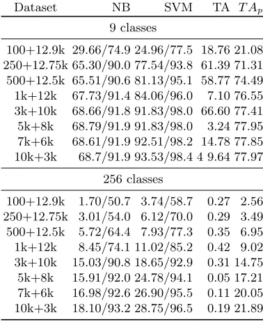
Table 6: Testing results, semi-supervised learning, DPAcontest v4, label spread-ing, (ACC/AUC)
Dataset NB SVM TA T Ap
9 classes
100+12.9k 29.66/74.9 24.96/77.5 18.76 21.08 250+12.75k 65.30/90.0 77.54/93.8 61.39 71.31 500+12.5k 65.51/90.6 81.13/95.1 58.77 74.49
1k+12k 67.73/91.4 84.06/96.0 7.10 76.55
3k+10k 68.66/91.8 91.83/98.0 66.60 77.41
5k+8k 68.79/91.9 91.83/98.0 3.24 77.95
7k+6k 68.61/91.9 92.51/98.2 14.78 77.85
10k+3k 68.7/91.9 93.53/98.4 4 9.64 77.97
256 classes
100+12.9k 1.70/50.7 3.74/58.7 0.27 2.56
250+12.75k 3.01/54.0 6.12/70.0 0.29 3.49
500+12.5k 5.72/64.4 7.93/77.3 0.35 6.95
1k+12k 8.45/74.1 11.02/85.2 0.42 9.02
3k+10k 15.03/90.8 18.65/92.9 0.31 14.75
5k+8k 15.91/92.0 24.78/94.1 0.05 17.21
7k+6k 16.98/92.6 26.90/95.5 0.11 20.05
Table 7: Testing results, semi-supervised learning, DPAcontest v2, self-training, (ACC/AUC)
Dataset NB SVM TA T Ap
9 classes
100+12.9k 14.45/51.2 18.67/49.2 7.30 16.95 250+12.75k 12.32/50.3 20.84/50.3 0.50 16.20 500+12.5k 12.90/52.1 21.40/49.1 1.39 17.55
1k+12k 12.73/52.5 25.21/50.6 0.40 14.86
3k+10k 7.02/52.4 25.00/51.5 1.47 12.43
5k+8k 10.34/54.2 25.51/50.2 15.03 11.80
7k+6k 10.95/52.2 26.04/50.2 1.67 11.05
10k+3k 10.18/50.8 26.24/50.3 8.33 8.62
256 classes
100+12.9k 0.55/50.0 0.50/50.0 0.50 0.40
250+12.75k 0.68/50.0 0.51/50.3 0.50 0.41
500+12.5k 0.55/50.2 0.45/50.3 0.59 0.44
1k+12k 0.50/50.4 0.38/50.4 0.59 0.51
3k+10k 0.42/50.3 0.48/50.1 0.36 0.41
5k+8k 0.45/50.5 0.42/50.0 0.41 0.40
7k+6k 0.62/50.7 0.64/50.3 0.39 0.44
10k+3k 0.51/51.1 0.54/50.3 0.43 0.41
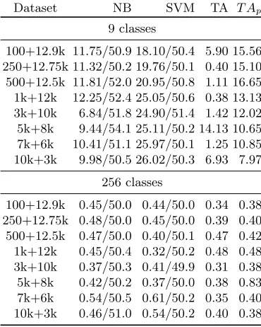
Finally, Table 8 gives results for DPAcontest v2 with Label spreading. The behavior is quite similar to that of self-training but we see somewhat worse ac-curacies throughout all scenarios. Smaller number of measurements for 9 classes have higher accuracies than using more measurements but this is due to a lack of labeled examples of all classes which corresponds to easier problem since then the classification process has less classes to choose from. When considering 256 classes, again we see AUC equal to 50% in a number of cases, which strongly suggests that high level of noise coupled with many classes does not work well for semi-supervised learning if the number of labeled measurements is low.
5
Discussion
5.1 Lessons Learned
In this section, we give more general conclusions on semi-supervised learning that can be transferred to other SCA settings. Although some of those considerations are quite natural and confirmed in different application domains [9], we translate them to the context of SCA.
Table 8: Testing results, semi-supervised learning, DPAcontest v2, label spread-ing, (ACC/AUC)
Dataset NB SVM TA T Ap
9 classes
100+12.9k 11.75/50.9 18.10/50.4 5.90 15.56 250+12.75k 11.32/50.2 19.76/50.1 0.40 15.10 500+12.5k 11.81/52.0 20.95/50.8 1.11 16.65
1k+12k 12.25/52.4 25.05/50.6 0.38 13.13
3k+10k 6.84/51.8 24.90/51.4 1.42 12.02
5k+8k 9.44/54.1 25.11/50.2 14.13 10.65
7k+6k 10.41/51.1 25.97/50.1 1.25 10.85
10k+3k 9.98/50.5 26.02/50.3 6.93 7.97
256 classes
100+12.9k 0.45/50.0 0.44/50.0 0.34 0.38
250+12.75k 0.48/50.0 0.45/50.0 0.39 0.40
500+12.5k 0.47/50.0 0.40/50.1 0.47 0.42
1k+12k 0.45/50.4 0.32/50.2 0.48 0.48
3k+10k 0.37/50.3 0.41/49.9 0.31 0.38
5k+8k 0.42/50.2 0.37/50.0 0.38 0.83
7k+6k 0.54/50.5 0.61/50.2 0.35 0.40
10k+3k 0.46/51.0 0.54/50.2 0.40 0.38
capabilities of semi-supervised learning and improvements can be easily reached. DPAcontest v2 is significantly more difficult for semi-supervised learning but still reasonable improvements are observed. For scenarios where we cannot observe any improvements, the number of measurements needs to be increased or number of class decreased in order to gain improvements for semi-supervised learning.
Number of Classes The less there are classes, the easier for SSL to be successful. Still, if there are enough examples per class it does not seem that having a lot of classes (e.g., 256 classes) presents a problem for SSL (granted, if the level of noise is not too high and the number of measurements is high enough). Interesting cases are when the number of labeled examples are so low that we do not have all class examples successfully trained. Then, the accuracy in the classification can go up since the problem becomes simpler due to decreased number of classes. Such increase in performance unfortunately does not help in SCA context.
Threshold Levels In the semi-supervised learning, unlabeled examples are clas-sified and help to augment the behavior of a classifier in the testing phase. The question is whether all predicted labels should be considered or only those with the highest probabilities. We opted to use the second approach in order to avoid adding too many measurements that are misclassified. Then, one needs to select what measurements to actually use, i.e., to decide which measurements have sufficiently high enough probabilities. Unfortunately, this threshold is an addi-tional parameter one needs to tune but that process is relatively straightforward and robust. Starting with very high probability threshold and decreasing it until some measurements are classified seem to be a good option. All experiments suggest that using a threshold level that is lower than strictly necessary will not significantly deteriorate the behavior of a classifier.
Generalizations of Models The aim of the training phase is to obtain a model that generalizes well to unseen data. In general, we see that SSL is able to build strong models that can compete with supervised learning. Our experiments show that having misclassified measurements from semi-supervised learning can be even beneficial in obtaining such models. Indeed, adding “noise” can help prevent models from over-training (thus, overfitting).
Choice of Classifiers In our experiments we use three classifiers in the semi-supervised phase. Later, in the semi-supervised phase we use two classifiers belonging to ML family as well as TA. The obtained results show differences (as expected) in the performance with respect to the choice of classifiers. Those differences occur both in semi-supervised and supervised learning. Still, the stable behavior across a number of testing scenarios suggest that different families of classifiers can be used with good results.
5.2 Future Work
Since the results obtained in our experiments show that semi-supervised learning can significantly improve SCA, we believe there is a number of research avenues of high interest. We considered four scenarios with respect to the number of classes and the amount of noise. The first straightforward extension of this paper would be to experiment further in those directions and consider more relevant scenarios appearing in SCA. For example, when using simulated data, a threshold for the signal-to-noise ratio in combination with the number of profiling measurements could be defined.
Besides that, we considered a number of cases with respect to the amount of traces but all scenarios had upper limit of 20 000 traces in total for training and testing phases. Since the results show that semi-supervised learning is of highest help when the number of labeled traces is significantly lower than the number of unlabeled traces, extending the search with the respect to the number of traces could produce even more interesting results. As an example, we could consider scenarios where the number of labeled traces is extremely small (100 labeled traces like we used here, or even less) while the number of unlabeled examples is much larger, for example 30 000 or even more.
Next, in this paper we considered two paradigms from semi-supervised learn-ing domain: self-trainlearn-ing and graph-based algorithms. Those techniques can be considered as older examples from the semi-supervised learning domain. It would be interesting to investigate whether the more recent (and often considered more powerful) techniques could still be more beneficial for SCA. For further inves-tigation we note especially the Co-training class of algorithms that falls under the paradigm of multi-view learning, first introduced by Blum and Mitchel [24]. The idea is that, when starting from a small training set with two different views (feature spaces)X1 andX2, the method iteratively re-trains a pair of different classifiers, one for each view, adding at each step the unlabeled samples that are classified with high confidence by one of the classifiers. As an example, instead of having one classifier working with all 50 features, we could divide it into two random sets of 25 that form two different views for co-training.
As already stated, from the semi-supervised learning we did not take all measurements but only those with the highest probabilities. Although our inves-tigations show such an approach gives very good results we could easily imagine improving it further. There, we could consider not only the highest probabilities but also the distribution of probabilities. As an example, the question is whether we should more believe in results where the best prediction is 60% while the sec-ond best is 40% (meaning all the other probabilities are zero) or when the best prediction is 50% while all the other ones are below 10%. Although in the first scenario the accuracy for the best prediction is higher, the difference between the first and the second best is larger in the second scenario, which we believe is the behavior we could use to further improve classification.
the measurements of the DPAcontest are attained by measuring the same device, therefore besides extrinsic noise, no differences in the distributions between the profiling and the attacking phase should be expected. In a real-world scenario, however, two different devices should be measured which may result in (slightly) different distributions (see e.g., [25, 26]). From our perspective, using a semi-profiled learning approach might greatly benefit the efficiency of the attack as the model is learned on both distributions, instead of only the one from the profiling device. This may open a new field of future investigation that consider real-world attacking scenarios.
In the semi-supervised phase, we used machine learning classifiers to obtain new labeled measurements but there is no reason why not to also use pooled template attack. Consequently, we plan to investigate the scenario where pooled template attack is used as the classifier in the self-training paradigm.
6
Conclusions
This paper investigates how to use semi-supervised learning in the context of SCA and whether such a paradigm is useful in realistic scenarios. Previously, in the SCA community, profiled side-channel analysis has been considered as a strict two-step process, where only the profiled model is transferred between the two phases. Most of the time it is assumed that the profiling phase is unbounded and the attacker has unrestricted possibilities and full knowledge of the profiling device. Contrary to that, the capabilities in the attacking are highly restricted and the attacker can only measure a very limited number of traces.
In this paper, we explore the scenario in which an attacker is more restricted in the profiling phase. For example, we adapt the concept of the “lunchtime” attack, in which the attacker might only gain access to a device where he has (or a group of people have) full knowledge of the underlying properties (e.g., secret key) during lunch time. Then again, in the attacking phase he may be not as restricted as he has the possibility to choose any device (similar to the one he used for profiling). Accordingly, the scenario changes to a (very) restricted profiling phase with labeled samples and a more unrestricted attacking phase with unlabeled samples. Clearly, in general, the attacker is not unhindered in exchanging all possible information between the profiling and attacking phase. In particular, he could use the additional available information given from the attacking measurements already to build the profiled model.
using additional samples from the attacking phase improved the estimation of the covariance matrices which resulted in improvements of up to 58%. Naturally, the higher the amount of samples in the profiling phase the less influential are the additional added unlabeled samples from the attacking phase. Note that, in the scenarios with no increase in accuracy, the behavior is not deteriorated compared to supervised learning (standard profiling phase), which makes semi-supervised learning a general technique to be considered.
Besides stating our results in these investigated contexts, we discuss more general conclusions on semi-supervised learning for SCA. This should help to transfer our observations to other settings in SCA. From our perspective, semi-supervised learning can significantly improve SCA and we are confident there is a number of research directions for future work as discussed in the previous section.
References
1. Heuser, A., Rioul, O., Guilley, S.: Good is Not Good Enough — Deriving Optimal Distinguishers from Communication Theory. In Batina, L., Robshaw, M., eds.: CHES. Volume 8731 of Lecture Notes in Computer Science., Springer (2014) 2. Lerman, L., Poussier, R., Bontempi, G., Markowitch, O., Standaert, F.:
Tem-plate attacks vs. machine learning revisited (and the curse of dimensionality in side-channel analysis). In Mangard, S., Poschmann, A.Y., eds.: Constructive Side-Channel Analysis and Secure Design - 6th International Workshop, COSADE 2015, Berlin, Germany, April 13-14, 2015. Revised Selected Papers. Volume 9064 of Lec-ture Notes in Computer Science., Springer (2015) 20–33
3. Heuser, A., Zohner, M.: Intelligent Machine Homicide - Breaking Cryptographic
Devices Using Support Vector Machines. In Schindler, W., Huss, S.A., eds.:
COSADE. Volume 7275 of LNCS., Springer (2012) 249–264
4. Cagli, E., Dumas, C., Prouff, E.: Convolutional Neural Networks with Data Aug-mentation Against Jitter-Based Countermeasures - Profiling Attacks Without Pre-processing. In Fischer, W., Homma, N., eds.: Cryptographic Hardware and Em-bedded Systems - CHES 2017 - 19th International Conference, Taipei, Taiwan, September 25-28, 2017, Proceedings. Volume 10529 of Lecture Notes in Computer Science., Springer (2017) 45–68
5. Maghrebi, H., Portigliatti, T., Prouff, E.: Breaking Cryptographic Implementa-tions Using Deep Learning Techniques. In Carlet, C., Hasan, M.A., Saraswat, V., eds.: Security, Privacy, and Applied Cryptography Engineering - 6th International Conference, SPACE 2016, Hyderabad, India, December 14-18, 2016, Proceedings. Volume 10076 of Lecture Notes in Computer Science., Springer (2016) 3–26 6. Heyszl, J., Ibing, A., Mangard, S., Santis, F.D., Sigl, G.: Clustering Algorithms for
Non-Profiled Single-Execution Attacks on Exponentiations. In: CARDIS. Lecture Notes in Computer Science, Springer (November 2013) Berlin, Germany.
8. Schwenker, F., Trentin, E.: Pattern classification and clustering: A review of par-tially supervised learning approaches. Pattern Recognition Letters37(2014) 4–14 9. Chapelle, O., Schlkopf, B., Zien, A.: Semi-Supervised Learning. 1st edn. The MIT
Press (2010)
10. Bengio, Y., Delalleau, O., Le Roux, N.: Efficient Non-Parametric Function
Induction in Semi-Supervised Learning. Technical Report 1247, D´epartement
d’informatique et recherche op´erationnelle, Universit´e de Montr´eal (2004) 11. Hall, M., Frank, E., Holmes, G., Pfahringer, B., Reutemann, P., Witten, I.H.:
The WEKA Data Mining Software: An Update. SIGKDD Explor. Newsl.11(1)
(November 2009) 10–18
12. Mitchell, T.M.: Machine Learning. 1 edn. McGraw-Hill, Inc., New York, NY, USA (1997)
13. Begum, S., Chakraborty, D., Sarkar, R.: Data Classification Using Feature Se-lection and kNN Machine Learning Approach. In: 2015 International Conference on Computational Intelligence and Communication Networks (CICN). (Dec 2015) 811–814
14. Pedregosa, F., Varoquaux, G., Gramfort, A., Michel, V., Thirion, B., Grisel, O., Blondel, M., Prettenhofer, P., Weiss, R., Dubourg, V., Vanderplas, J., Passos, A., Cournapeau, D., Brucher, M., Perrot, M., Duchesnay, E.: Scikit-learn: Machine
Learning in Python. Journal of Machine Learning Research12(2011) 2825–2830
15. Choudary, O., Kuhn, M.G.: Efficient template attacks. In Francillon, A., Rohatgi, P., eds.: Smart Card Research and Advanced Applications - 12th International Conference, CARDIS 2013, Berlin, Germany, November 27-29, 2013. Revised Se-lected Papers. Volume 8419 of LNCS., Springer (2013) 253–270
16. Friedman, J.H., Bentley, J.L., Finkel, R.A.: An Algorithm for Finding Best Matches
in Logarithmic Expected Time. ACM Trans. Math. Softw.3(3) (September 1977)
209–226
17. Vapnik, V.N.: The Nature of Statistical Learning Theory. Springer-Verlag New York, Inc., New York, NY, USA (1995)
18. Platt, J.: Fast Training of Support Vector Machines using Sequential Minimal Optimization. In Schoelkopf, B., Burges, C., Smola, A., eds.: Advances in Kernel Methods - Support Vector Learning. MIT Press (1998)
19. Keerthi, S.S., Shevade, S.K., Bhattacharyya, C., Murthy, K.R.K.: Improvements to
Platt’s SMO Algorithm for SVM Classifier Design. Neural Comput.13(3) (March
2001) 637–649
20. Keerthi, S.S., Lin, C.J.: Asymptotic Behaviors of Support Vector Machines with
Gaussian Kernel. Neural Comput.15(7) (July 2003) 1667–1689
21. Witten, I.H., Frank, E., Hall, M.A.: Data Mining: Practical Machine Learning Tools and Techniques. 3rd edn. Morgan Kaufmann Publishers Inc., San Francisco, CA, USA (2011)
22. TELECOM ParisTech SEN research group: DPA Contest (2nd edition) (2009–
2010)http://www.DPAcontest.org/v2/.
23. TELECOM ParisTech SEN research group: DPA Contest (4thedition) (2013–2014)
http://www.DPAcontest.org/v4/.
24. Blum, A., Mitchell, T.: Combining Labeled and Unlabeled Data with Co-training. In: Proceedings of the Eleventh Annual Conference on Computational Learning Theory. COLT’ 98, New York, NY, USA, ACM (1998) 92–100
-30th Annual International Conference on the Theory and Applications of Crypto-graphic Techniques, Tallinn, Estonia, May 15-19, 2011. Proceedings. Volume 6632 of Lecture Notes in Computer Science., Springer (2011) 109–128