P-Values maximized over a confidence set for the nuisance parameter

1

Introduction

Testing problems are often complicated by the presence of a nuisance parameter vector

. Consider first a model in which there is no nuisance parameter. Suppose the data

X

have a probability distribution

P

defined in terms of a parameter

, and we wish to test the simple hypothesis

H

0 :

=

0. If the test statistic

T

is used to test

H

0

and if large values of

T

give evidence against

H

₀, then for an observed value

T

=

t

, the

p-value is

p

=

P

0(

T

t

).

Now consider a model with a nuisance parameter

. The distribution of

X

has two parameters,

and

. We still wish to test

H

0 :

=

0, but this hypothesis is no

longer simple, because the value of

is unspecified. Using a test statistic as above, the p-value is now

p

=sup

P

0

;

(

T

t

). (See, for example, Bickel and Doksum (1977), pp.

171-172). Unfortunately, the need to calculate the sup

has complicated the problem.

This complication is usually handled in one of three ways. First, in some problems it can be shown that, for all values of

t

, the sup

is always attained at a particular value

0. In this case the p-value is simply

p

=

P

0

;

0(

T

t

), and the parameter(

0

;

0)is called

the least favorable configuration. For example, in common one-sided testing problems, the boundary of the null hypothesis space is least favorable.

A second way to handle the unknown

is to choose judiciously a test statistic

T

(that usually depends on estimated values of

) whose distribution under

H

₀ does not depend on

. That is,

T

is ancillary under

H

0. Then,

P

0

;

(

T

t

) is the same for all

so

calculation of the sup

is avoided. For example, in normal means problems we replace unknown variances with sample variances and use t or F distributions to account for the estimated variances.

A third method to handle the unknown

is to condition on the value of a statistic

S

that is sufficient for

under

H

0. Then the conditional distribution of any statistic, given

S

, does not depend on

(under

H

0), and the p-value is taken to be

p

=

P

0(

T

t

j

S

=

s

).

For example, in a two by two contingency table with common “success” probability

under

H

0, one can condition on the marginals (a sufficient statistic for

under

H

0) and

All three methods replace the calculation of the sup

by the calculation of a single probability, and each method can result in avalidp-value, i.e., a statistic

p

such that, under the null hypothesis,

P

(

p

)

;

for each

2[0

;

1]

:

(1)

We call a statistic that satisfies (1) a valid p-value because it can be used in the standard way to define a level -

test. That is, consider the test that rejects the null hypothesis if and only if

p

. Then under the null hypothesis,

P

(reject null)=

P

(

p

)

. That is, the test so defined is a level -

test.

In many situations, however, none of the above three methods is satisfactory. For example, the value of

at which the sup

occurs may depend on the value

t

in a complicated way. Also, exact distributional results are often not available for statistics with estimated parameters. And finally, it may not be possible to find an appropriate sufficient statistic to condition upon.

In this paper we want to consider a different approach for obtaining valid p-values. Suppose that a valid p-value

p

(

0) may be calculated when the true value

0 of

the nuisance parameter vector

is known. Here it should be noted that the calculation of

p

(

0) does not have to be based on the same test statistic for different values of

0.

Indeed, the test statistic may depend directly on the assumed known value of

₀. All that is needed is that, for each value of

0,

p

(

0) is a statistic that satisfies (1). If

0 is

not known, then a valid p-value may be obtained by maximizing

p

(

)over the parameter

space of

. That is,

p

sup=sup

p

(

)clearly satisfies (1).

The use of

p

sup has two potential difficulties, one computational and the other

propose as a p-value

p

( ^

), where ^

is an estimate of

(usually the maximum likelihood estimate). But p-values defined in this way may not be valid. See the computations of Storer and Kim (1990).

A valid p-value that addresses both of the above concerns is defined as follows. Let

C

be a 1?

confidence set for the nuisance parameter when the null hypothesis

is true. Intuition suggests that we might be able to restrict the maximization to the set

C

. Indeed we show below that

p

=sup

2

C

p

(

)+

(2)

is an alternative valid p-value. This p-value may be preferred to

p

supon computational

grounds (due to maximizing over bounded sets) and on statistical principles (restricting interest to likely regions of

). The value of

and the confidence set

C

should of course be specified before looking at the data. Note that

p

is never smaller than

. So, in practice,

will be chosen rather small, such as .001 or .0001. If

p

is to be used to define a level -

test, then

must be less than

to obtain a useful test.

We will first give the theoretical justification for

p

in the following lemma. The rest of the paper is a series of illustrative examples. The first example, a pedagog-ical example, concerns tests about a normal mean when the variance is unknown. The remaining, more-realistic examples are about two by two contingency tables, the Behrens-Fisher problem, nonparametric testing for skewness, and nonparametric test-ing for scale differences.

2

Validity of

p

Lemma. Suppose that

p

(

) satisfies (1) for any assumed known value

. Let

C

satisfy

P

(

2

C

) 1?

, if the null hypothesis is true. Let

p

be given by (2). Then,

p

is a valid p-value.

Proof. Suppose the null hypothesis is true. Denote the true but unknown

by

0. If

>

, then since

p

is never smaller than

,

P

(

p

)=0

. If

, then

P

(

p

) =

P

(

p

;

0 2

C

)+

P

(

p

;

0 2

P

(

p

(

0)+

;

0 2

C

)+

P

(

02

C

)

P

(

p

(

0)

?

)+

?

+

=

:

The first inequality follows because sup

2

C

p

(

)

p

(

0)when

0 2

C

.

3

Examples

Example 1. Pedagogical example about a normal mean. Let

X

1

;:::;X

n

be a

random sample from a normal population with mean

and variance

2_{. We consider}

testing

H

0 :

=

0 versus

H

1 :

6=

0, where

0 is a fixed value and

2 is the nuisance

parameter. We consider this familiar example to illustrate our method, not to offer a serious contender to the usual t-test.

If

2 were known, we could use the test statistic

Z

= p

n

(

X

?

0)

=

, where

X

is the sample mean. Then the two-sided p-value would be

p

(

2

)=2(?j

z

obsj)

;

where

z

obs is the value of the test statistic calculated from the data, and (

z

) is the

standard normal cumulative distribution function. As a confidence interval for

2_{, we}

will use the upper confidence bound given by

C

= (

2_{: 0}

2

(

n

?1)

s

2

2

)

;

where

s

2 _{is the sample variance and}

2

is the 100

percentile of a chi-squared distri-bution with

n

?1 degrees of freedom. The valid p-value we propose is

p

= sup

22

C

p

(

2

)+

= sup

22

C

2(?j

z

obsj)+

:

Sincej

z

obsjis a decreasing function of

, the sup

C

occurs at the upper endpoint. (This is why we chose to use an upper confidence bound.) Thus

p

=2(?j

z

maxj)+

, where

z

max is the test statistic calculated with

2=(

n

?1)

s

2

=

2

In this example, the test statistic

Z

depends on the value of the nuisance pa-rameter, a possibility mentioned in Section 1. Also, in this example, the p-value

p

sup,

although valid, is useless because it always has the value 1, sincej

z

obsj!0 as

!1.

So the fact that maximization is restricted to

C

when calculating

p

is of critical im-portance in getting a reasonable answer.

This example is a bit unusual in that the sup

_C

can be calculated exactly. In many cases this will need to be calculated numerically.

This example is also unusual in that the exact size of the test based on

p

can be calculated. Suppose we reject

H

0 if

p

. Then the actual size of the test is

P

(

p

) =

P

(2(?j

Z

maxj)+

)

=

P

((?j

Z

maxj)(

?

)

=

2)

=

P

(?j

Z

maxj

z

(

?

)

=

2

)

= 2

P

(

T

q

(

n

?1)

=

2

z

(

?

)

=

2 )

;

where

T

has a Student’s t distribution with

n

?1 degrees of freedom and

z

is the

100

percentile of a standard normal distribution. It can be shown that

q

(

n

?1)

=

2

converges to 1 as

n

goes to infinity. So the actual size of the test, which is at most

since the p-value is valid, converges to

?

.

Example 2. Two by two contingency table with independent binomial sampling.

Consider a two by two contingency table consisting of two independent binomial sam-ples, 14 “successes” out of 47 trials for group 1 and 48 “successes” out of 283 trials for group 2. This data appeared in Table 1 of Emerson and Moses (1985) who obtained it from Taylor et al. (1982). We consider here the usual two by two table chi-squared statistic

Z

2 =

(^

1?

^2) 2

^

(1?

^)( 1

n

1

+ 1

n

2

)

;

where

^ =(

n

1

^1+

n

2

^2)

=

(

n

1+

n

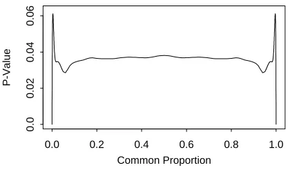
2) and

^1 and

^2 are the sample proportions in the two

Common Proportion

0.0 0.2 0.4 0.6 0.8 1.0

0.0

0.02

0.04

0.06

P-Value

Figure 1: Exact p-values for the two by two table chi-squared statistic. Calculations are from independent binomial distributions with common proportion

.

binomial proportions

1 and

2 as a function of the unknown common

under the null

hypothesis

H

0 :

1 =

2 =

. The p-value

p

(

) for a fixed value of

is computed from

the binomial distribution as

p

(

)= X

b

(

x

; 47

;

)

b

(

y

; 283

;

)

where

b

(

x

;

n;

)is the binomial probability of

x

successes in

n

trials with success

prob-ability

, and the sum is over all pairs (

x;y

) of

x

successes from group 1 and

y

suc-cesses from group 2 that give a

Z

2 value bigger than or equal to the

Z

2 = 4

:

346

value calculated from this data. The usual, unconditional p-value for this problem is

p

sup = sup

2[0

;

1]

p

(

) =

:

061. Suissa and Shuster (1985) discuss this p-value and

recommend it as an appropriate p-value for this problem.

Looking at Figure 1, however, it would seem natural to restrict the region over which the maximization takes place to a region around the null maximum likelihood estimate ^

= (48 +14)

=

(283+47) =

:

188. A .999 confidence interval for

under

the null hypothesis is given by [.123,.267] (e.g., Casella and Berger, 1990, p. 499). Numerically calculating the sup of

p

(

) over this interval yields the value .036. Thus,

the new p-value is

p

:

001=

:

036+

:

001 =

:

037. This improvement in the p-value is not

unusual since the maximum over[0

;

1]often occurs near 0 or 1, far from the estimated

In fact, the program EXACTB by Shuster (1988) will compute the maximum of

p

(

) over a .999 confidence interval, and report it as a p-value. But the program

documentation does not provide any theory to justify this approach. Also, the value reported is just the maximum, not the maximum plus

as in (2). So the reported p-value may not be valid. As an aside, we note that EXACTB will also compute

p

sup.

But for this data, the value computed by EXACTB was

p

sup =

:

038. Apparently, the

maximization routine failed to detect the spikes in

p

(

) near 0 and 1. But the spikes

are real and the correct value is .061, as we reported above.

Example 3. Behrens-Fisher problem. The classical Behrens-Fisher problem has two independent samples

X

1

;:::;X

m

and

Y

1

;:::;Y

n

from normal distributions with

means

1 and

2 and variances

12 and

22. The null hypothesis is

H

0 :

1 =

2 where

2

1 is not assumed equal to

22.

Best and Rayner (1987) recently reaffirmed the practical value of the Welch solu-tion based on

t

w

=

X

?

Y

r

s

2 1

m

+

s

2 2

n

;

where

X

,

Y

,

s

2

1, and

s

22 are the usual sample means and sample variances, and critical

values are obtained from a

t

distribution with estimated degrees of freedom. Numerous studies have shown, however, that the Welch solution can be slightly liberal. In other words the corresponding p-value does not satisfy (1) for certain combinations of

m

and

n

and

=

=

2 2

=

21.

Here we can use our approach along with

t

w

to get a valid p-value since, under

H

0 :

1 =

2, the distribution of

t

w

depends only on the ratio of variances

=

2 2

=

12.

Although the distribution of

t

w

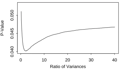
is not simple, we can easily simulate from normal distributions to get a p-value for each value of

. Figure 2 shows the results for a data set with sample means 0

:

0 and 6

:

225 and sample variances 18 and 78 (an example taken from Barnard (1984)). A .999 confidence interval for

obtained from the F distribution of

s

2

1

=s

22 is (.32,38.72). On this interval the maximum two-sided p-value is

.048 so that

p

:

001=

:

048+

:

001=

:

049. Since the p-value was obtained from 1,000,000

Ratio of Variances

0 10 20 30 40

0.040

0.045

0.050

P-Value

Figure 2: Estimated p-values for Welch’s t as a function of the ratio of variances

. Number of Monte Carlo replications = 1,000,000.

comparison purposes note that the Welch solution p-value is .041, the pooled

t

p-value is .065, and the Behrens-Fisher p-value is .050.

Another way to use our approach in this problem follows from the quantity

t

(

)=

X

?

Y

r

( 1

m

+

n

) (

m

?1)

s

2

1+(

n

?1)

s

2 2

=

m

+

n

?2

;

given by Fisher (1939, p. 176). For a given value of

,

t

(

) has a

t

distribution with

m

+

n

?2 degrees of freedom under

H

0. Thus, we might consider using our approach

with

t

(

)and this latter

t

distribution. The appropriate

p

(

)is easy to calculate and has

intuitive appeal. Unfortunately this

p

(

) is much more sensitive to changes in

than

the simulation

p

(

) based on

t

w

. We do not display the results for

p

(

) but note that

p

:

001=

:

233+

:

001=

:

234 and

p

:

01=

:

15+

:

01=

:

16. Clearly the method based on

t

w

is

superior.

In fact, we believe that there is a general principle here concerning our methods to the effect that one should use statistics such as

t

w

whose null distribution depends on the nuisance parameter rather than use pivotal quantities such as

t

(

) which are

functions of the nuisance parameter but whose null distributions do not depend on the nuisance parameter.

Behrens-Fisher problem, although Barnard (1984, Sec. 6) claims that Robinson (1976) has shown that the Behrens-Fisher solution p-value is valid. It is not clear to us that Robinson (1976) has actually proved such a result. But from a practical view we must point out that neither our solution nor the Behrens-Fisher solution are likely to be robust to nonnormality since they both use the F distribution of

s

2

1

=s

22.

The three previous examples were parametric problems where the nuisance pa-rameter

was confined to (0

;

1), [0,1] and (0

;

1), respectively. Now we turn to more

ambitious semi-parametric problems where

is a location parameter belonging to

(?1

;

1), but in addition, there is a second infinite dimensional nuisance

parame-ter corresponding to an unknown distribution function. This is really not much harder than the previous examples, however, because we can handle this latter nuisance pa-rameter using classical permutation test methods. That is, for each given value of

, we will obtain a permutation p-value and then carry on as in Examples 2 and 3.

Example 4. Testing for skewness with unknown location. We have a single iid sample

X

1

;:::;X

n

and wish to test whether the

X

’s are symmetrically distributed about

some unknown

. Formally the null hypothesis is

H

0 :

F

(

+

x

) = 1?

F

((

?

x

) ?

) all

x

2(?1

;

1),

F

and

unknown. A variety of good test statistics have been proposed for

this problem, but no finite sample valid p-values have been given. In fact Schuster and Barker (1987) have proposed bootstrap methods because even approximate validity has been so elusive.

For illustration purposes we shall consider two simple statistics. The first is the sample standardized third moment

p

b

1=

m

3

=m

3

=

2 2

;

where

m

k

= P

(

X

i

?

X

)

k

=n

. D’Agostino, Belanger, and D’Agostino (1990) discuss the

use of

p

b

1 as a test for normality, but there has been no valid method for using it as

a test of asymmetry. For example, Randles, et al. (1980) show that the appropriate standardization of

p

b

1 by an estimate of its asymptotic standard deviation results in a

normal test which is extremely liberal for a variety of symmetric distributions.

T

=

=

^

;

^

where

^is the

U

-statistic estimate of

=

P

(

X

1+

X

2

>

2

X

3)?

P

(

X

1+

X

2

<

2

X

3) and

^ is

the corresponding estimate of standard deviation.

T

is asymptotically normal for any symmetric

F

, but Table 2 of Randles et al. (1980) shows that using normal or t critical values results in a test which is approximately valid in small samples but which can be liberal for certain symmetric

F

s.

Our method in this situation is as follows. For given

, a valid p-value can be obtained by calculating the statistic of interest for each of the 2

n

possible samples of the formj

X

1?

j

;:::;

j

X

n

?

j. The permutation p-value is just the proportion of these

values which are greater than or equal to the statistic calculated from the original

n

observations. Since 2

n

is often a very large number, we typically randomly sample from the set of possible permutations.

The second ingredient of our method is a confidence interval for

. The simplest in-terval is the exact confidence inin-terval for the median (which equals

under

H

0) given by

(

X

(

l

)

;X

(

n

?

l

+1)

), where

X

(1)

X

(

n

)are the order statistics and

=(1

=

2)

n

?1

P

l

?1

i

=0

ni

(see David, 1981, Sec. 2.5).

To illustrate, we consider the sample of

n

= 62 cholesterol values given in

D’Agostino, Belanger, and D’Agostino (1990). Figure 3 shows estimated right-tailed p-values versus

for

p

b

1 and

T

based on 10,000 random permutations. Using

l

=18 in

the above confidence procedure, we get

=

:

000497, and so a .9995 confidence interval

for

under

H

0is(

X

(18)

;X

(45)

)=(220

;

267)resulting in

p

:

0005=

:

0370+

:

0005 =

:

038 for p

b

1and

p

:

0005=

:

0177+

:

0005=

:

018 for

T

. Use of the random permutations (instead of

all 262 permutations) introduces a standard error of about((0

:

03)(0

:

97)

=

10

;

000) 1

=

2

=

0

:

0017.

The triples statistic for this data is

T

=2.501, and using a

t

distribution with

n

=62

degrees of freedom as suggested by Randles et al. (1980), we get an approximate right-tailed p-value of .0075. Since

:

018

=:

0075=

:

2

:

4, we might say that there is a 2.4 "cost"

factor in this case to obtain the valid p-value of .018, rather than an approximate value. Using

p

b

1and the approximation given by D’Agostino, Belanger, and D’Agostino

Theta

200 220 240 260 280 300

0.0

0.02

0.04

(a) Standardized 3rd Moment

P-Value

Theta

200 220 240 260 280 300

0.0

0.02

0.04

(b) Triples Statistic

Figure 3: Estimated p-values for tests of skewness for cholesterol data. Number of random permutations = 10,000.

distribution. Here though,it is unfair to compare with the valid p-value of .038 since the null class of all symmetric distributions is much bigger than that of the set of normal distributions.

The range of variation of the p-values in Figure 3 is much larger for

p

b

1 than

for

T

. We believe that the difference is due to the robustness of

T

compared to that of p

b

1. That is, the sample third moment is very sensitive to outliers and to small

changes in distributional shape. The triples

T

is an average of indicator functions and insensitive on a large scale to such changes although wiggles do occur because of the discontinuities caused by the indicator function. A second difference between

p

b

1 and

T

is the fact that

T

is studentized and

p

b

1 is not. A plot of p-values for

^in place of

T

(not displayed) is qualitatively similar to Figure 3b and suggests that studentization is not a major cause of differences between Figures 3a and 3b.

Example 5. Testing for scale differences in two populations with unknown

loca-tions. Consider two iid samples

X

1

;:::;X

m

and

Y

1

;:::;Y

n

with distribution functions

F

((

x

?

1)

=

1) and

F

((

x

?

2)

=

2), respectively. The null hypothesis is

H

0 :

1 =

2;

F

,

1and

1 are unknown. This model is not identifiable, but an equivalent description in

which all parameters are identifiable is for the

X

s and

Y

s to have distribution functions

F

(

x

) and

F

((

x

?)

=

), respectively. The null hypothesis is then

H

0 :

= 1;

F

and

As in Example 4, there are numerous good test statistics in the literature for this problem but none accompanied by valid finite sample p-values. Actually, one can randomly pair the data in each sample and create differences

X

i

?

X

j

and

Y

i

?

Y

j

, thereby

eliminating the unknown locations. Rank and permutation tests on the differences then yield valid tests, but the loss in power due to the random pairing makes this approach unsuitable. A good review of test statistics and practical methods is found in Conover et al. (1981).

If the difference in locationswere known, we could subtractfrom each of the

Y

s, pool the

X

s and transformed

Y

s, and carry out the standard permutation approach. That is, we compute a statistic

T

for each of the

m

+

n

m

distinct permutation data sets (

X

1

;:::;X

m

;

Y

1

;:::;Y

n

) drawn without replacement from the set(

X

1

;:::;X

m

;Y

1?

;:::;Y

n

?). The permutation p-value is then the proportion of these values which

are greater than or equal to the statistic calculated from the original data.

For illustration we consider the weight gain of a group of

m

= 30 control rats

and of a second group of

n

=20 rats whose diet included calcium EDTA. The observed

values for the control group are

34, 22, 51, 33, 20, 32, 35, 24, 13, 22, 26, 38, 34, 30, 20, 30, 25, 32, 36, 22, 26, 28, 31, 28, 32, 31, 28, 28, 31, 31,

and for the treated group are

9, 23, 16, 13,-13, 32, 10, 26, 14,-24, 8, 29, 24, 27, 22, 2, 19, 21, 27, -1.

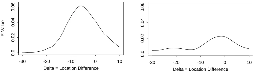
Figure 4 shows the estimated p-values for j

log

(

s

1

=s

2)j and j

log

(

g

1

=g

2)j, where

s

2 1

and

s

2

2 are the sample variances and the

g

i

are robust scale estimators with the form

g

1=

1

M

?[

M

(

:

25)]

M

?[

M

(

:

25)] X

i

=1

Z

(

i

)

;

and the

Z

(

i

)are the

M

=

m

(

m

?1)

=

2 ordered values ofj

X

j

?

X

k

j. These trimmed versions

of Gini’s Mean Difference were studied in Janssen, Serfling, and Veraverbeke (1987) and subsequently found to have good efficiency and robustness properties.

An exact 1?

confidence interval forunder

H

0may be obtained by inverting any

Delta = Location Difference

-30 -20 -10 0 10

0.0

0.02

0.04

0.06

(a) Ratio of Sample Standard Deviations

P-Value

Delta = Location Difference

-30 -20 -10 0 10

0.0

0.02

0.04

0.06

(b) Ratio of Robust Standard Deviations

Figure 4: Estimated p-values for tests of scale for weight gain data. Number of random permutations = 10,000.

Wilcoxon rank sum statistic which has the form[

D

(

k

)

;D

(

l

)

)where

D

(1)

;:::;D

(

mn

) are the

ordered differences of the form

Y

j

?

X

i

(see Randles and Wolfe, 1979, p. 180). The .999

confidence interval for the above data is [-24,-3]. This leads to

p

:

001=

:

062+

:

001=

:

063

for the variance-based statistic of Figure 4a and to

p

_:

₀₀₁=

:

022+

:

001 =

:

023 for the

robust statistic of Figure 4b. The standard errors of these p-values are about .002 due to using 10,000 random permutations.

Asymptotic arguments are given in Boos, Janssen, and Veraverbeke (1989) which justify the use in large samples of

p

(

^

), where ^

is estimated from the data. For

example,

Y

?

X

= 14

:

2?29

:

1 = ?14

:

9 leading to

p

(?14

:

9) =

:

018 and .006 from

Figures 4a and 4b, respectively. Taking the ratios .063/.018 and .023/.006 suggests a "cost" factor around 3 to 4 for getting a valid p-value for this data in place of an asymptotic approximate p-value.

We also note that, as in Example 4, the p-value for the nonrobust statistic based on sample variances is much more sensitive to changes in , ranging from .0012 to

.062 over2[?24

;

?3], while the robust statistic based on

g

1 and

g

2 ranges from .005

4

Summary

Nuisance parameters may be handled in a variety of ways in testing problems. In this paper we have introduced a new method for modifying the standard definition of a p-value given by

p

= sup

P

0

;

(

T

t

) to allow for taking the supremum over a

confidence interval for

instead of over the whole parameter space of

.

The new method is not intended to supplant standard methods for handling nui-sance parameters, when those methods give tractable answers. But our examples suggest that the new method can indeed give improved procedures, as in the case of the two by two contingency table using the

Z

2 _{statistic. In other situations the new}

method can give finite-sample level -

tests where none previously existed.

REFERENCES

Barnard, G. (1984), “Comparing the Means of Two Independent Samples,” Applied

Statistics, 33, 266-271.

Best, D. J., and Rayner, J. C. W. (1987), “Welch’s Approximate Solution for the Behrens-Fisher Problem,”Technometrics, 29, 205-210.

Bickel, P. J., and Doksum, K. A. (1977), Mathematical Statistics: Basic Ideas and

Selected Topics, San Francisco: Holden-Day, Inc.

Boos, D., Janssen, P., and Veraverbeke, N. (1989), “Resampling from Centered Data in the Two-Sample Problem,” Journal of Statistical Planning and Inference, 21, 327-345.

Casella, G., and Berger, R. L. (1990),Statistical Inference, Pacific Grove, CA: Wadsworth.

Conover, W. J., Johnson, M. E., and Johnson, M. M. (1981), “A Comparative Study of Tests for Homogeneity of Variances, with Applications to the Outer Continental Shelf Bidding Data,” Technometrics, 23, 351-361.

Using Powerful and Informative Tests of Normality,”The American Statistician, 44, 316-321.

David, H. A. (1981),Order Statistics, 2nd Ed., New York: John Wiley.

Emerson, J. D., and Moses, E. M. (1985), “A Note on the Wilcoxon-Mann-Whitney Test for 2 x k Ordered Tables,”Biometrics, 41, 303-309.

Fisher, R. A. (1939), “The Comparison of Samples with Possibly Unequal Variances,”

Annals of Eugenics, 9, 174-180.

Janssen, P., Serfling, R., and Veraverbeke, N. (1987), “Asymptotic Normality of U-Statistics based on Trimmed Samples,”Journal of Statistical Planning and Inference, 16, 63-74.

Randles, R. H., and Wolfe, D. A. (1979), Introduction to the Theory of Nonparametric

Statistics, New York: John Wiley.

Randles, R. H., Fligner, M. A., Policello, G. E., II, and Wolfe, D. A. (1980), “An Asymp-totically Distribution-Free Test for Symmetry versus Asymmetry,” Journal of the

American Statistical Association, 75, 168-172.

Robinson, G. K. (1976), “Properties of Student’s

t

and of the Behrens-Fisher Solution to the Two Means Problem,”Annals of Statistics, 4, 963-971.

Schuster, E. F., and Barker, R. C. (1987), “Using the Bootstrap in Testing Symmetry versus Asymmetry,” Communications in Statistics - Simulation & Computation, 16, 69-84.

Shuster, J. (1988), “EXACTB: Exact Unconditional P-Values for the 2x2 Binomial Trial,” Research Assistance Corp, Gainesville, Fl.

Storer, B. E., and Kim, C. (1990), “Exact Properties of Some Exact Test Statistics for Comparing Two Binomial Proportions,”Journal of the American Statistical Associa-tion, 85, 146-155.

Suissa, S., and Shuster, J. (1985), “Exact Unconditional Sample Sizes for the 2x2 Binomial Trial,”Journal of the Royal Statistical Society, Ser. A, 148, 317-327.