DOI: 10.1534/genetics.108.099275
Methods for Human Demographic Inference Using Haplotype Patterns
From Genomewide Single-Nucleotide Polymorphism Data
Kirk E. Lohmueller,*
,†,1Carlos D. Bustamante
†and Andrew G. Clark*
*Department of Molecular Biology and Genetics and†Department of Biostatistics and Computational Biology, Cornell University, Ithaca, New York 14853
Manuscript received December 5, 2008 Accepted for publication February 19, 2009
ABSTRACT
We propose a novel approximate-likelihood method to fit demographic models to human genomewide single-nucleotide polymorphism (SNP) data. We divide the genome into windows of constant genetic map width and then tabulate the number of distinct haplotypes and the frequency of the most common haplotype for each window. We summarize the data by the genomewide joint distribution of these two statistics—termed the HCN statistic. Coalescent simulations are used to generate the expected HCN statistic for different demographic parameters. The HCN statistic provides additional information for disentangling complex demography beyond statistics based on single-SNP frequencies. Application of our method to simulated data shows it can reliably infer parameters from growth and bottleneck models, even in the presence of recombination hotspots when properly modeled. We also examined how practical problems with genomewide data sets, such as errors in the genetic map, haplotype phase uncertainty, and SNP ascertainment bias, affect our method. Several modifications of our method served to make it robust to these problems. We have applied our method to data collected by Perlegen Sciences and find evidence for a severe population size reduction in northwestern Europe starting 32,500–47,500 years ago.
A
major goal of evolutionary genetics is to infer the demographic history of a population. This is traditionally done by fitting a population genetic model to sequence data taken from a sample of individuals. The population genetic model often includes param-eters allowing for changes in population size or population structure with or without migration. Such parameters are interesting in their own right, but are critical to define a proper ‘‘null model’’ that can be used to find ‘‘unusual’’ genes that may be targets of positive or negative selection (Jensen et al. 2005). Additionally, a proper demographic model is important for assessing genomewide patterns of positive and negative selection (Boyko et al. 2008; Lohmueller et al.2008).Methods have been developed that make full use of sequence data to infer demographic parameters (Griffithsand Tavare´1994; Kuhneret al.1995). These methods are computationally intensive and are imprac-tical for all but the smallest data sets. Thus, researchers have turned to methods based on summary statistics (reviewed in Marjoram and Tavare´ 2006). Summary statistics can be quickly calculated from the data and then be used to infer model parameters using either a
likelihood or approximate Bayesian computation (ABC) framework (for example, Wall 2000a; Fagundes et al. 2007). The key for successful application of this approach is to find summaries of the data that contain enough information about the demographic parameters of in-terest. One of the most successfully used summary statistics for population genetic inference, the site frequency spectrum (SFS) (Nielsen2000; Adams and Hudson 2004; Caicedo et al. 2007; Hernandez et al. 2007b), is a sufficient statistic for the full data if the single-nucleotide polymorphisms (SNPs) are unlinked. How-ever, in reality, all SNPs are not unlinked. The amount of information in the data lost by ignoring the correlations among SNPs, or linkage disequilibrium (LD), in de-mographic inference is an open question, but recent theoretical work suggests that it may be nonnegligible (Myerset al.2008).
An additional complication to using the SFS for demographic inference is that many genomewide ge-netic variation data sets in humans contain SNPs that were discovered through sequencing a small number of individuals. The discovered SNPs were then genotyped in a larger set of individuals, sometimes in a different population than was used for SNP discovery. Since this SNP discovery process will lead to preferential sampling of intermediate-frequency alleles, the SFS computed from SNP genotype data will differ substantially from the true SFS (Nielsen et al.2004; Clark et al.2005). Progress has been made to analytically correct the SFS Supporting information is available online athttp://www.genetics.org/
cgi/content/full/genetics.108.099275/DC1.
1Corresponding author:102F Weill Hall, Cornell University, Ithaca, NY 14853. E-mail: [email protected]
for ascertainment bias when the SNP discovery process is known (Nielsenet al.2004), but often this is not the case. More problematic is the situation where SNPs were discovered by resequencing individuals in one popula-tion, but then are genotyped in a second population. It remains an open question as to how well the SNPs discovered in the first population are representative of genetic diversity in the second population. Several authors have suggested that statistics based on combina-tions of multiple SNPs, or haplotypes, will be less susceptible to ascertainment bias than single-SNP fre-quencies or heterozygosities (Conradet al.2006). How-ever, while this suggestion is encouraging, as yet there has not been extensive investigation into the precise ascer-tainment conditions under which this is true.
It is known that haplotype patterns and LD can be affected by both recombination and demographic history (Pritchard and Przeworski 2001), making these measures useful statistics for inference. Many recent studies have assumed a demographic model (often the standard neutral model) and then used either LD or haplotype patterns to estimate recombina-tion rates (Wall2000a; Hudson2001; Liand Stephens 2003; McVean et al. 2004; Myers et al. 2005). Other studies have taken the opposite approach and assumed that the recombination rate is known and then used LD or haplotype patterns to estimate demographic param-eters (Reichet al.2001; Innanet al.2005; Voightet al. 2005; Schaffneret al.2005; Lebloisand Slatkin2007; Tenesa et al. 2007). The way in which haplotype in-formation has been used for demographic inference is quite variable among studies. For example, Reichet al. (2001) examined how well several different demo-graphic models predicted the observed decay of pair-wise LD in humans, rather than estimating the model parameters. Francoiset al.(2008) and Thorntonand Andolfatto (2006) used ABC to estimate model parameters in Arabidopsis and Drosophila, respectively. However, summaries based on the distribution of the number of haplotypes were only one of several summary statistics considered, and it is unclear how much in-formation came from the haplotype inin-formationvs.the other single-SNP diversity measures. While Anderson and Slatkin(2007) and Lebloisand Slatkin(2007) developed methods that use haplotype information exclusively to fit a population split followed by growth model, their model is quite restrictive and allows inference only of one free parameter, the number of founding lineages. Thus, there has not been a system-atic investigation as to the utility of haplotype informa-tion for inference in general, parameter-rich models, such as those involving population expansions and bottlenecks.
In this article we propose an approximate-likelihood method to estimate parameters in complex demo-graphic models from genomewide SNP genotype (rather than full resequencing) data, using the joint
distribution of the number of haplotypes and frequency of the most common haplotype in windows across the genome. We provide extensive simulations evaluating the performance of our method for growth and bottleneck models. These results indicate that a great deal of information regarding demographic history is captured by these two summary statistics. We also extensively test the robustness of our method to many practical problems with genetic data sets in humans. Specifically, we show that for many realistic SNP discov-ery protocols and levels of population divergence, our method is relatively robust to SNP ascertainment bias. We also found that our method is sensitive to recombi-nation rate variation across the genome (as many haplotype-based summaries will be), and we incorpo-rate a model of recombination incorpo-rate variation into the inference scheme. Finally, since haplotype phase is often ambiguous, we provide a practical approach to circumvent this problem. We applied our method to genomewide SNP genotype data generated by Perlegen Sciences (Hinds et al. 2005). Using the CEU sample (consisting of individuals from Utah with northwestern European ancestry), we find evidence for a recent population bottleneck in northwestern Europe.
METHODS
Summary statistics: We summarize the genomewide data by the joint distribution of two haplotype statistics calculated from windows across the genome. Our method requires that we have a genetic map of the organism in question. Using this map, we divide the genome into windows of fixed genetic map distance, cwindow. The parametercwindowis tunable to the diversity and recombination rates of the organism under study. We chose to divide the genome into nwindow nonover-lapping windows using genetic map distance so that each window will have the same expected amount of recombination within it and, consequently, the same expected number of haplotypes (Wall2000a).
second population. Since rare SNPs are more likely to be population specific, and consequently not equally ascertained in all populations, we include only those SNPs with minor allele frequency (MAF)$10%.
Having selected a subset of intermediate-frequency SNPs from each window, we can compute the number of distinct haplotypes as well as the count of the most common haplotype in a sample of n chromosomes. The HCN statistic is the genomewide joint distribu-tion of these two statistics. Specifically, let X ¼ ðX1;1;X1;2;. . . ;X1;l;X2;1;. . . ;X2;l;. . . ;Xk;1;. . .;Xk;lÞ, where Xij denotes the number of windows having i haplotypes where the most common haplotype has count j out of n. In principle, k¼l¼n; however, in practice, we bin intervals in the HCN statistic for the inference so that fewer simulation replicates will be needed to obtain an accurate estimate of the expected HCN (see below), and thus there are fewer thann2bins in the HCN statistic. Ideally, we wish to integrate over all possible sets of nsnp SNPs within each window when constructing the HCN statistic. However, this is not
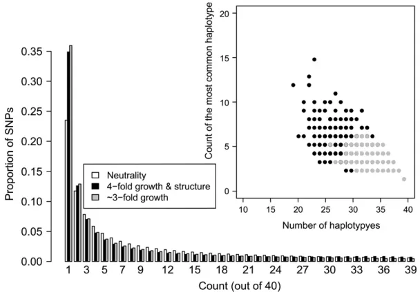
computationally feasible, so we generate 10 random matrices, each using a different randomly selected set of nsnpSNPs from each window. We then average these 10 matrices as our finalXmatrix to be used for inference. This is done to reduce Monte Carlo variance resulting from selecting a single set of SNPs. An example of the HCN statistic for several demographic models is shown in Figure 1.
number of haplotypes is more informative about overall population size than is the count of the most common haplotype (compareNcur¼10,000 toNcur¼5000), as expected, since larger populations have a higher pop-ulation recombination rate, r¼4Nec than smaller populations, resulting in a larger number of haplotypes per window (Wall 2000a). Note that because we selected nsnp SNPs with MAF$10% per window, the fact that the larger population has a higher value ofu does not inflate the observed number of haplotypes per window. A recent bottleneck results in an intermediate number of haplotypes, but the stronger signature of the bottleneck is the excess proportion of windows where the most common haplotype is at unusually high frequency. These patterns are due to an elevated rate of coalescence during the bottleneck, which, for some simulated windows, results in there being fewer lineages available to recombine. A recent population expansion also results in an intermediate number of haplotypes, but without an increase in the number of windows where the frequency of the most common haplotype is unusually high.
The HCN statistic contains no information about how different haplotypes within a window are from each other. To add this information, we also considered another summary statisticHpair, the distribution across the genome of the average number of pairwise differ-ences between haplotypes. For allðn
2Þpairs of haplotypes within a given window, we simply counted the number of SNPs (which could range from 0 tonsnp) where the two haplotypes differed and counted the average.Hpair is the vector giving the number of windows having a given number of average pairwise differences. We show (supporting information, File S1 and Figure S1) that this statistic is not robust to SNP ascertainment bias and do not use it in further analyses.
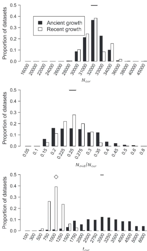
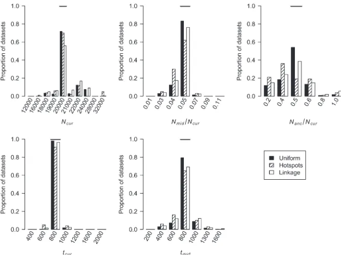
Demographic models: We consider two different single-population demographic models. These models and their associated parameters are shown in Figure 2. Figure 2A shows a two-epoch model that is used for modeling population growth. Here there are three parameters to estimate: the current population size, Ncur; the ancestral population size,Nmid; and the time that growth has occurred,tcur. Figure 2B shows a three-epoch model that has five free parameters: the current population size, Ncur; the population size during the bottleneck,Nmid; the ancestral population size,Nanc; the time when the bottleneck started (going backward in time),tcur; and the duration of the bottleneck,tmid. All times are in units of generations. We note that although these models (and all models in population genetics) are arbitrary simplifications of the true demographic history, the hope is that they capture some essential features of population history.
Fitting models to data: Since the observed HCN statistic follows a multinomial distribution, we fit de-mographic models to the data using an
approximate-likelihood approach (see Weiss and Von Haeseler 1998; Wall 2000a; Fearnhead and Donnelly 2002; Plagnol and Wall 2006). We define p¼ ðp1;1; p1;2;. . .;p1;l;p2;1;. . .;p2;l;. . .;pk;1;. . .;pk;lÞ, where pij is the probability that a window hasihaplotypes where the most common haplotype is at countj. The approx-imate-likelihood function for the demographic param-eters (Q) can be written as
LðQÞ Y k
i¼1
Yl
j¼1 pXij
ij : ð1Þ
We use the coalescent with recombination (Hudson 1983, 2002) to findpijfor the demographic parameter combination of interest. We simulatezreplicates using the demographic parameters of interest (Q) and r ¼ 4Ncurcwindow. We estimate the matrixpas the proportion of simulation replicates falling in a particular bin of the HCN statistic. Formally, define the indicator function Iðw;i;jÞto be equal to 1 if simulation replicatewhasi haplotypes and the count of the most common haplo-type isj, and equal to 0 otherwise. Then
pij¼
Pz
w¼1Iðw;i;jÞ
z : ð2Þ
Since we selectnsnp SNPs from each window,u does not explicitly enter into these simulations. Therefore, instead of setting an arbitrary value of u, and then randomly selecting nsnp SNPs, we use the ‘‘fixed S approach’’ (Hudson1993) to add mutations onto the ancestral recombination graph (ARG). Specifically,nsnp mutations are randomly placed onto each simulated ARG such that these SNPs will have MAF $10%. To reduce Monte Carlo error, this process is repeated 10 times for each ARG. Each time, we evaluateIðw;i;jÞand increment the appropriate bin ofp. Note that we record 10 differentpmatrices and after the desired number of simulation replicates, we keep the average of the 10p matrices as our final matrix. This is an approximate-likelihood function since we are approximatingpusing simulations, rather than calculating it exactly, and we also treat all windows of the genome as being mutually independent.
approximating the likelihoods by simulation and the simulation variance may be nonnegligible, misleading deterministic hill-climbing approaches. The number of grid points and number of simulation replicates used to maximize the approximate-likelihood function vary among analyses and are given below.
Since variation in recombination rates at a fine scale can affect the HCN statistic, we have added a model of recombination hotspots into our inference method. We describe the parameters used for specific instances below. Since each window of the genome corresponds to the same genetic map distance (cwindow), the number of base pairs per window will differ among windows. In our simulations to find p, we select the size of the window in base pairs (denotedL) from the observed distribution of physical distances. We then setr, the per base pair recombination rate, to be constant across the window such thatrLwill givecwindow. We then simulate an ARG in the normal manner with recombination rate rL, but then, similar to the method used by Li and Stephens(2003), we model hotspots by changing the relationship between physical and genetic distance. Informally, the parts of the window where hotspots occur are assigned fewer base pairs and consequently have a lower probability of a SNP occurring in them than windows with lower recombination rates.
Simulations to evaluate performance:We tested the performance of our method by simulating data under three different demographic models: (1) ancient pop-ulation growth, (2) recent poppop-ulation growth, and (3) a recent population bottleneck. The parameter values for these models are shown in Figures 3–6. These models were chosen because of their relevance to human demographic history. For each model we simulated data sets (500 for models assuming uniform recombination rates and 100 for models with recombination hotspots), each consisting of 2000 independent 250-kb windows in a sample of 40 chromosomes wherem¼13108/bp/ generation. Note that when generating test data sets, we placed a Poisson number of mutations onto the gene-alogies in the usual fashion (Hudson1983), rather than using the fixedSapproach as we did for the simulations used to estimatep. We selected a subset of 20 SNPs (nsnp¼ 20) with MAF$10% from each window and constructed the observed HCN statistic for each data set. We repeated this process 10 times for each data set and used the average HCN statistic for inference. For computational efficiency, we performed the coalescent simulations to estimate p over a grid of parameters (3780 and 20,580 parameter combinations for the growth and bottleneck models, respectively) once for each demographic and recombination model and stored the values to be used on subsequent data sets. The grid points used for each parameter are shown as the breaks in Figures 3–6. For each grid point we used 104 coalescent simulations to approximate the likeli-hood. Using a representative data set, we then selected
at least the top 103grid points and ran an additional 105 replicates, and for points near the maximum-likelihood estimates (MLEs), we ran an additional 106replicates. Due to computational constraints, these grids were not as dense as those used to estimate parameters in the Perlegen data.
For all data sets and demographic models, the total amount of recombination within each window simu-lated was 0.25 cM (i.e.,cwindow¼0.25 cM). However, we also considered a model with five recombination hot-spots present at random locations throughout each window. Each hotspot was 2 kb in size. The recombina-tion rate (centimorgans per base pair) of each hotspot was drawn from a gamma distribution (shape ¼ 0.5, scale¼23106). We then rescaled the recombination rate of each hotspot such that 80% of the total amount of recombination in the window occurs within hotspots. We then assumed this model of recombination hotspots when inferring demographic parameters. The test data sets were generated using the program msHOT (Hellenthaland Stephens2007).
Our method assumes that all windows in the genome are independent of each other. To assess the perfor-mance of our method when the windows are not independent, we simulated an additional 500 data sets using the same bottleneck model withcwindow¼0:25 cM. Here the 2000 windows within each data set were from 300 independent sets of 6 or 7 contiguous windows. All windows were treated as independent in the inference. While for most of the simulations we assumed that there was no error in estimated recombination rates (i.e.,ˆcwindow¼cwindow), we also determined what effect errors in the estimated genetic map had on our ability to accurately infer demographic parameters. Specifically, we simulated data sets under the same bottleneck model described above, but here instead of having ˆcwindow¼ cwindow¼0:25 cM, we drewcwindowfor each window from a gamma distribution (shape¼10, scale¼0.025). From this distribution,10% of windows havecwindow,0.155 and 10% of windows havecwindow. 0.355. We then inferred demographic parameters when incorrectly fixingˆcwindow¼0:25 cM. We also correctly incorporated errors into the genetic map by drawingˆcwindowfor each simulation replicate from the same gamma distribution used to generate the data.
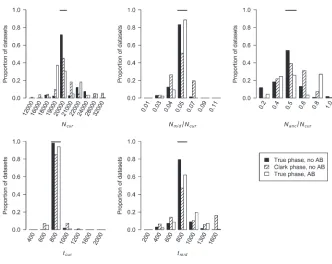
phasing algorithm proposed by Clark(1990). If there are no individuals heterozygous at zero or one of the nsnpSNPs within a window or if there are genotypes that show no relation to known phased haplotypes, we arbitrarily assigned phase to a random individual and then used these two haplotypes to infer the rest. While this process may seem arbitrary, it can be done consis-tently both in the observed and in the simulated data sets. To make the method as computationally efficient as possible, we used only one ordering of the individuals. We assessed the performance of this approach by treating the simulated haplotypes in the test data sets as diploid genotypes and ‘‘phased’’ them using the parsimony method. For each simulation replicate to estimatepwe also phased the simulated data using the same parsimony method.
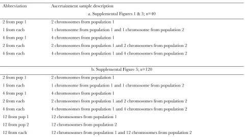
Since we found that the HCN statistic constructed using SNPs that were discovered in a SNP discovery sample$8 chromosomes was very similar to the HCN statistic with complete SNP ascertainment (Figure S3, Figure S4, Figure S5, Table S1, and File S1), we ex-amined how ascertainment bias affected parameter estimates. Specifically, for the bottleneck model de-scribed above, we simulated a genotype sample ofn¼40 and an additional SNP discovery sample of 6 chromo-somes. Since the Perlegen SNPs were discovered using a multiethnic panel (Hinds et al. 2005), we included a SNP discovery sample of an additional 6 chromosomes from a second population (Ncur ¼ 10,000) that 5000 generations ago split from the population that un-derwent the bottleneck. To construct the HCN statistic from these simulated data sets, we considered only SNPs with MAF $10% in the genotype sample that were variable in the 12-chromosome ascertainment panel. To infer parameters, we assumed there was no ascertain-ment bias (i.e., we used the same lookup tables forpthat were described above that assumed complete SNP ascertainment).
Analysis of Perlegen data:We applied our method to fit a bottleneck model to the CEU population geno-typed by Perlegen Sciences (Hinds et al. 2005). We chose to use this population since there is previous evidence of a bottleneck in this population (e.g., Marth et al.2004; Voightet al.2005), and all SNPs that were discovered by the Perlegen resequencing arrays were later genotyped in the CEU sample, without regard to LD status. We note that HapMap phase II specifically did not genotype SNPs that were in high LD in the Perlegen study, and this ascertainment criterion complicates the analysis of those data (seediscussion). We considered only autosomal (not X chromosome or mtDNA) SNPs with MAF $10% in both the CEU and the African-American samples. Since our simulations of ascertain-ment bias suggest that SNPs needed to have been discovered from discovery sample sizes .2 chromo-somes, we used only those SNPs that were discovered in Perlegen’s resequencing arrays of the multiethnic
di-versity panel (type ‘‘A’’ SNPs). There were 615,415 SNPs that fit both of these criteria. We used Clark’s parsimony phasing algorithm to phase haplotypes in both the real data and the simulation replicates to generate p. For each population and in each window of the genome, we selected 10 random subsets of nsnp SNPs and con-structed 10 different HCN statistics. We then used the average HCN statistic for inference.
We then setcwindow¼0.25 cM andnsnp¼20. We used the LDhat genetic map (InternationalHapmapC on-sortium 2007) to define windows since the deCODE map (based on pedigrees; Konget al. 2002) does not have sufficient resolution for the scale of 0.25 cM (Myers et al. 2005). Since the quality of the genetic map used to divide the genome into windows can affect the inference, we drewˆcwindowfrom a gamma distribu-tion (shape¼10, scale¼0.025) to model errors in the genetic map. This distribution has a mean of 0.25 and a variance of 0.00625. For the CEU data,nwindow¼8833. We used a hotspot model similar to that of Schaffner et al.(2005; termed the ‘‘Schaffner hotspot model’’). All hotspots had width of 2 kb. For each simulated window, hotspots occurred at random intervals drawn from a gamma distribution (shape ¼ 0.3, scale ¼ 8500/0.3), giving a mean spacing of 8.5 kb (variance of2.413
108). Then the recombination rate (cM/2 kb) of each hotspot was drawn from another gamma distribution (shape ¼ 0.3, scale ¼ˆcwindow=0:3L), where L is the physical size of the simulated window. In practice, L was drawn from the empirical distribution of physical distances for thenwindowwindows. We then rescaled the recombination rate in the hotpots such that 88% of ˆcwindowoccurs within hotspots. The amount of recombi-nation occurring outside of hotspots is then equal to 0:12ˆcwindow. Figure S6 and Figure S7 show that this hotspot model matches the mean, the standard de-viation, and the overall distribution (tabulated across all windows of the genome) of the observed inter-SNP genetic map distances quite well.
In addition to the Schaffner hotspot model described above, we also directly used the estimated fine-scale LDhat genetic map (InternationalHapmapC onsor-tium2007) as a guide to how recombination rates vary within windows (termed the ‘‘empirical hotspot’’ model). To do this, for each simulation replicate to estimate p, we selected one of the 8833 windows at random and used the corresponding LDhat genetic map to delimit the relationship between genetic and physical distance for that replicate. We smoothed the map by allowing the recombination rate to change only at points.500 bp and.0.0001 cM apart. We note that this hotspot model does not match the observed inter-SNP genetic distances as well as the Schaffner hotspot model does (Figure S6andFigure S7).
empirical hotspot model. We used 12,500 simulation replicates for all points, 105replicates for at least the top 4000 points, and finally 106replicates for at least the top 500 points. We found approximate 95% confidence intervals (C.I.’s) for single parameters using asymptotic theory (i.e., the C.I. included points ,1.92 log-likeli-hood units from the maximum), with linear interpola-tion of the profile-likelihood curve to find points not directly simulated.
RESULTS
Performance on simulated data: Figure 3 shows the distribution of the approximate MLEs of the three growth model parameters for simulated data sets under ancient growth (solid bars) and recent growth (open bars). In both cases, the method is relatively unbiased for all three parameters. For ancient growth,Ncuris estimated most accurately andtcurthe least. For recent growth, all three parameters are equally accurate, although for any given parameter, the MLE is the true value40% of the time. Note that the variance in the distribution of MLEs fortcuris much higher for ancient growth as compared to recent growth (making it the least precise as well as the least accurate). Table 1 shows that for both growth scenarios in 100% of the data sets, the true parameter values were within the asymptotic 95% C.I.’s (,3.9 log-likelihood units) around the MLEs. Additionally, in.95% of the data sets, the one-dimensional 95% C.I.’s for all three parameters from the profile-likelihood curves contain the true parameter values.
We also estimated the five parameters for a bottleneck model in simulated data sets. Figure 4 shows the dis-tribution of the MLEs for the five bottleneck parame-ters. For the case of uniform recombination and ˆcwindow¼cwindow¼0:25 cM, the mode of the distribu-tion of the MLEs for each parameter is at the true value of the parameter. The distribution of MLEs is tightest forNmid/Ncurandtcurand broadest forNanc/Ncur. This suggests that the recent bottleneck greatly alters haplo-type patterns such that its timing and severity can be accurately estimated, but so much so that less informa-tion about the ancestral, prebottleneck populainforma-tion size (Nanc/Ncur) remains. Furthermore, the method appears to be relatively unbiased since it over- and under-estimates the true parameter value roughly equally. Table 1 shows that 99.8% of the time, the true parameter values are within the asymptotic 95% C.I.’s (within 5.5 log-likelihood units around the MLEs).
We next evaluated whether our method could accu-rately estimate demographic parameters in the pres-ence of recombination hotspots (seemethodsfor the recombination hotspot model used). Figure 4 shows that when properly modeling recombination hotspots, we are able to accurately estimate the five bottleneck model parameters. Note that the distributions of the
true parameter values are ,5.5 log-likelihood units from the MLEs.
The simulations described above assumed that the windows in each data set were independent. In practice, the windows may be contiguous along the genome and
thus are not independent. We examined the perfor-mance of our method on simulated data sets where some of the windows were linked. Figure 4 shows that the distributions of the MLEs for certain parameters have greater variance than when the windows are TABLE 1
Comparison of MLEs to the true parameter values for simulated data sets
Model
Mean llMLEs
llTrutha
Max llMLEs
llTruthb
% MLEs¼ truthc
Coverage of multi dimensional
95% C.I.’sd
Coverage of one-dimensional
95% C.I.’se
% points outside 95% C.I.’sf
Ancient growth
ˆcwindow¼cwindow¼0:25 cM 0.631 3.47 3.0 100.0 99.87 94.79 Recent growth
ˆcwindow¼cwindow¼0:25 cM 0.437 3.09 22.6 100.0 99.93 98.84 Bottleneck
ˆcwindow¼cwindow¼0:25 cM 0.363 6.31 47.4 99.8 99.52 99.87
Hotspotsg 0.505 3.43 17.0 100.0 99.80 99.65
Linkage 0.732 8.30 29.8 99.4 98.48 99.87
ˆcwindow¼0:25 cM,cwindow gamma 136.685 179.07 0.0 0.0 8.36 99.98
ˆcwindowcwindow gamma 0.623 6.54 26.4 99.6 99.40 99.72
Clark’s phasing algorithmh 0.779 4.90 19.8 100.0 99.96 99.43
Ascertainment bias 1.998 12.65 14.6 94.0 97.64 99.86
a
The average overall data sets of the log-likelihood at the MLEs minus the log-likelihood of the true demographic parameters.
bThe maximum distance between the log-likelihood at the MLEs and the log-likelihood of the true demographic parameters. cThe proportion of data sets where the MLEs for all parameters were the true demographic parameters.
dThe proportion of data sets where the true parameter values were,3.9 or,5.5 log-likelihood units from the MLEs, for the
growth and bottleneck models, respectively.
eThe proportion of data sets where the true value of each parameter was,1.92 log-likelihood units from the MLE using the
profile log-likelihood curve, averaged over three or five parameters for the growth and bottleneck models, respectively.
fThe fraction of grid points (seeresults) having a log-likelihood.3.9 or.5.5 log-likelihood units, for the growth and
bot-tleneck models, respectively, from the MLEs.
g
Each window has five recombination hotspots, but for the whole windowˆcwindow¼cwindow¼0:25 cM.
h
Haplotype phase was inferred in the test data sets and simulations to estimatepusing Clark’s phasing algorithm (seemethods).
unlinked, which is not surprising since linked windows contain less information than independent windows. As shown in Table 1, in all cases except when errors in the genetic map are ignored or there is SNP ascertainment bias (see below), the true parameter values for.99% of the test data sets are within the asymptotic 95% C.I.’s (,3.9 and,5.5 log-likelihood units from the MLEs for growth and bottleneck models, respectively). This result suggests that the asymptotic C.I.’s may actually be conservative, since the true parameter values are con-tained within the interval .95% of the time. When examining data sets where some of the regions are linked, we find that for 99.4% of the time, the true values are,5.5 log-likelihood units from the MLEs (Table 1). Since in many cases, the 95% C.I.’s for individual parameters based on the profile log-likelihood curve also appeared conservative (Table 1), we assessed their coverage in the data sets with linkage. For each of the five parameters, the true parameter value is,1.92 log-likelihood units from the MLE in at least 96.8% of the data sets. These results suggest that for the level of nonindependence among windows, size of data sets, and parameter grid considered here, the asymptotic 95% C.I.’s remain conservative.
The above simulations assumed thatˆcwindow¼cwindow. In practice, ˆcwindow is estimated from a genetic map, based either on patterns of LD or on pedigrees. We next evaluated the performance of our method whencwindow is drawn from a gamma distribution to mimic errors in the estimated genetic map. We first assumed that ˆcwindow¼0:25 cM when running the inference (i.e., we ignored the errors in the genetic map). Figure 5 shows that our method performs poorly compared to the case where the genetic map is known with certainty. In
particular, it overestimatestcurandtmid. Due to the fact that some windows in the simulated data sets will have low recombination rates, these windows will have very few haplotypes and a high frequency of the most common haplotype because cwindow , 0.25 cM. Since we did not account for this in the inference, the method assumes that these low-diversity windows were due to a stronger (or longer) bottleneck. Table 1 shows that the true parameter values are nowhere near the MLEs in this case. If, however, during the inference, ˆcwindow for each window is drawn from the same gamma distribution that generated the data, the method performs substan-tially better (Figure 5), although not quite as well as when ˆcwindow¼cwindow¼0:25 cM. Likewise, 99.6% of the time, the true parameter values are,5.5 log-likelihood units from the MLEs. Note that, similar to what was seen for the case of recombination hotspots, on average, a smaller proportion of the parameter space (99.72%vs.99.87%) is.5.5 log-likelihood units from the MLEs whenˆcwindow andcwindowfollow a gamma distribution instead of being fixed at 0.25 cM.
certainty. Additionally, a smaller proportion of the parameter space is excluded (.5.5 log-likelihood units from the MLEs) when using Clark’s phasing algorithm as compared to known phase data (99.43% vs. 99.87%; Table 1). This finding illustrates that, compared to having phase-known haplotypes, some information is lost when computationally inferring haplotypes. However, the method appears reasonably unbiased, and in all simulated data sets the true parameter values are,5.5 log-likelihood units from the MLEs (Table 1).
To determine if we could accurately estimate bottle-neck parameters in the presence of SNP ascertainment bias, we simulated data sets where thensnp¼20 SNPs for each window were picked from those SNPs with MAF $10% in the genotype sample and were variable in the 12-chromosome SNP ascertainment sample. Figure 6 shows that for Nmid/Ncur, tcur, and tmid, our method performs very well even in the presence of SNP ascer-tainment bias. The distributions of the MLEs forNcurand Nanc/Ncur are more variable than when there is no ascertainment bias, and the modes of their distributions are not at the true parameter values, suggesting that MLEs of these parameters are less reliable in the presence of ascertainment bias. The 95% C.I.’s structed from the profile-likelihood curves remain con-servative forNmid/Ncur,tcur, andtmid, but forNcurthe 95% C.I. is no longer conservative (i.e., the true value is within the 95% C.I. only 91.8% of the time). Additionally, the five-dimensional 95% C.I. is also slightly anticonservative (Table 1). For larger data sets (consisting of 10,000 independent regions) the C.I.’s forNcurandNanc/Ncur and the five-dimensional C.I. become even more anti-conservative and the C.I. for tmid becomes slightly
anticonservative (not shown), likely due the fact that the ascertainment model is misspecified, which has a stronger effect as the size of the data set increases.
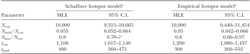
Inference of bottleneck parameters for the Perlegen CEU population: We fit the five-parameter bottleneck model to the Perlegen CEU population. Table 2 shows the MLEs and95% C.I.’s for the five parameters when using both the Schaffner model of recombination hotspots and the empirical hotspot model based on the LDhat genetic map.Figure S8shows that for both hotspot models, the HCNs generated using the MLE parameter estimates match the observed CEU HCN quite well. The current population size is estimated to be 10,000 when using both recombination models. There was a severe population size reduction (4.2–6.6% of the current size) lasting 260–552 generations (see Figure S9 for the two-dimensional profile-likelihood surface). The bottleneck ended (forward in time) 1017–1437 generations ago.
On the basis of the two-dimensional profile-likelihood surface (Figure S10), we estimate that the bottleneck began (tcur1tmid) 1500 generations ago—37,500 years, assuming 25 years/generation when using either hot-spot model. Notably, the oldest start time within the asymptotic 95% C.I. (3 log-likelihood units, for 2 d.f.) is 1600 generations, or 40,000 years for the Schaffner hotspot model, and 1900 generations (47,500 years) for the empirical hotspot model.
ery panel for the 615,415 SNPs used in constructing the HCN statistic used for demographic inference in the Perlegen CEU sample. We found that 11.8% of these SNPs were discovered by comparing fewer than eight chromosomes. We removed these SNPs and recom-puted the HCN statistic from the Perlegen CEU data (now with 8174 windows) and reestimated the bottle-neck parameters using the Schaffner recombination hotspot model. We found identical MLEs for the param-eters as in our original analysis.
DISCUSSION
We have proposed a flexible approximate-likelihood method to estimate demographic parameters using haplotype summary statistics. We have shown that accurate estimates of demographic parameters can be made using genomewide SNP data sets of practical size. To the best of our knowledge, this is one of the first studies to estimate parameters in a demographic model in a likelihood framework using haplotype patterns from genomewide SNP genotype data. Furthermore, we have addressed many complications that arise in the analysis of genomewide data, such as recombination rate heterogeneity, errors in the estimated genetic map, haplotype phase uncertainty, and ascertainment bias. Provided that good genetic maps are available, our method could be applied to SNP data from other species, such as dogs and cattle, to estimate domestica-tion bottleneck parameters.
One of the major disadvantages of our approach is its dependence on accurately modeling the distribution of recombination rates across the genome. Our simula-tions have shown that errors in the genetic map can cause poor performance. Therefore, we suggest apply-ing our method only when there is an accurate genetic map for the species in question. We suggest incorporat-ing a distribution on ˆcwindow to allow for errors in the estimated genetic map. However, as the quality and resolution of genetic maps continue to improve, the
utility and accuracy of our method will also continue to increase. For species where recombination rates vary at the fine scale, it is crucial to incorporate some model of recombination hotspots. Here for the Perlegen CEU data, we have implemented a parametric model as well as empirical estimates based on LD patterns. A similar influence of the assumed recombination rate on the de-mographic parameter estimates was noted in Thornton and Andolfatto(2006), who used the variance in the number of haplotypes across windows as one of their summary statistics. We recommend, as done in Thornton and Andolfatto (2006), using different recombina-tion models and then comparing the final results to assess how dependent the estimates are on the assumed recombination model. While the dependence of our method on accurate estimates of the recombination rate is not ideal, we point out that many previous methods in molecular evolution and population genet-ics are dependent on accurate estimates of the mutation rate and will be biased if erroneous estimates are used. We also assume that the genetic map remains constant over time and is the same across populations. Recombi-nation hotspots do not appear in the same locations in chimps and humans despite a high level of sequence identity (Ptaket al.2005; Winckleret al.2005). It has therefore been speculated that recombination hotspots are not permanent features of the genome and evolve on a timescale of at least tens of thousands of years ( Jeffreys et al.2005). However, it appears that the timescale over which many hotspots evolve is older than 100,000 years, and because this is long enough to alter patterns of LD, temporal changes in hotspots on this timescale will not have such a severe impact on our method. Hotspots that evolve over shorter timescales, or are population specific, may have a larger effect on our method. This effect is hard to quantify since the prevalence of rapidly evolving or population-specific hotspots, other than the existence of a few examples ( Jeffreys et al. 2005; Clark et al. 2007), remains largely unknown. Encouragingly, a recent article (Hellenthal et al. 2006) found that genotype-TABLE 2
Inferred bottleneck parameters for the CEU data set
Schaffner hotspot modela Empirical hotspot modelb
Parameter MLE 95% C.I. MLE 95% C.I.
Ncur 10,000 9,315–10,665 10,000 9,440–11,454
Nmid/Ncur 0.055 0.052–0.064 0.05 0.042–0.066
Nanc/Ncur 0.8 0.70–?c 0.8 0.66–0.97
tcur 1,100 1,017–1,140 1,200 1,086–1,437
tmid 400 360–475 300 260–552
MLEs and95% C.I.’s from the profile-likelihood curves for the five-parameter bottleneck model are shown.
a
The hotspot model is similar to that described by Schaffneret al.(2005) (seemethods).
b
The hotspot model is based directly on the LDhat genetic map.
c
specific recombination events would not substantially affect LD patterns, boding well for our method.
We have found that the HCN statistic constructed from computationally phase-inferred data differs from the true HCN. Simply treating the phase-inferred haplotypes as the true haplotypes will likely give biased parameter estimates. Thus, when analyzing data from unrelated individuals, it is important to consider errors induced in the phasing process. We suggest doing this by inferring phase for the coalescent simulations used to estimate HCN. Our simulations suggest that using Clark’s phasing algorithm works well for this purpose. However, some information is lost by this procedure (Figure 6; Table 1), and we therefore recommend, where available, using data from trios, where haplotype phase can be inferred with great accuracy, to maximize the information in the data.
It has been suggested (Conrad et al. 2006) that haplotype statistics may be less susceptible to SNP ascer-tainment bias than statistics based upon SNP frequencies. Here we have extensively investigated whether this holds true for the HCN andHpair statistics under a variety of demographic and ascertainment conditions. Encourag-ingly, we found that the HCN statistic is reasonably robust to SNP ascertainment bias provided that the SNP discov-ery sample is sufficiently deep. The reason for this is that we focus on subsets of common SNPs, rather than on rare SNPs. However, theHpairstatistic was very susceptible to ascertainment bias (Figure S1andFile S1), suggesting that all haplotype statistics are not equally affected by ascer-tainment bias, and it will be necessary to explicitly evaluate, as we have done here, whether ascertainment bias affects a particular haplotype statistic.
The sizes of the SNP discovery and genotype samples play an important role in determining the effect of ascertainment bias on the HCN statistic. Interestingly, generating the HCN from SNPs ascertained uniformly using two chromosomes of known ethnicity (as done by Keinanet al.2007) would result in a very different HCN statistic from that expected without ascertainment bias (Figure S3, Figure S4, and Figure S5), which would result in biased inference. Although not considered here, it is in principle possible to estimate the expected HCN statistic conditional on this particular ascertain-ment strategy, and application of such an estimate would reduce this bias.
We have found that SNP discovery sample sizes of at least 12 total chromosomes should be sufficient to result in the HCN statistic from ascertained SNPs to match the expected HCN when considering genotype samples of 40 or 120 chromosomes. Furthermore, we have shown that our method can reliably infer several bottleneck parameters when SNPs were ascertained in this manner. As the SNP discovery sample size increases, perfor-mance of our method will continue to improve and become closer to that for the case of no ascertainment bias, since a larger SNP discovery sample will capture
more of the SNPs in the genotype sample. These results are especially encouraging since Perlegen’s SNP discov-ery effort used 20–50 chromosomes, where12 chro-mosomes were of African-American ancestry, 12 chromosomes were of European ancestry, and the remainder were of Mexican-American, Asian-American, and Native American ancestry (Collins et al. 1998; Hindset al.2005).
Furthermore, we have found that the size of the SNP discovery sample is more important than whether or not the SNP ascertainment had been done in a particular population (see Figure S5). This suggests that SNPs ascertained in the Perlegen resequencing survey could be used to estimate demographic parameters in other populations not represented in the SNP discovery panel. It is worth noting that the two populations in our simulation study shown in Figure S5 split 5000 generations ago (125,000 years, assuming 25 years/ generation) with no subsequent migration and are thus more differentiated than many actual non-African populations that could be studied empirically.
It is important to note that the type of ascertainment bias studied here is due to the preferential genotyping of common SNPs. In all the analyses presented here, we assume that the genotyped SNPs were selected without regard to physical or genetic distance or LD patterns. Such an assumption is reasonable for the analyses of the Perlegen data presented here since Perlegen attempted to genotype all of the SNPs found in their SNP discovery process (Hindset al.2005). The assumption is not valid, however, for many of the ‘‘SNP chips’’ that preferentially selected SNPs on the basis of physical distance (in the case of Affymetrix 500K) or LD patterns (in the case of the Illumina platform; Eberle et al. 2007). Since the SNPs on these platforms are not a random subset of the total variation, using our method on such data will likely give misleading results. In principle, it should be possible to modify our method to model the SNP selection process in the inference, which would allow our method to be applied to the large-scale SNP genotype data sets that have been collected, such as the HGDP data set ( Jakobssonet al.2008; Liet al.2008). For the analysis of the CEU data, we used two different models of recombination rate variation. Overall, the results using both models are qualitatively similar, suggesting that our method is somewhat robust to minor misspecification of the recombination hotspot model. We also find that the one-dimensional 95% C.I.’s from the profile-likelihood curves overlap for all five parameters estimated (Table 2;Figure S11). Neverthe-less, the five-dimensional 95% C.I.’s do differ between the two recombination models, mainly due to the fact thattcur is greater under the empirical hotspot model than under the Schaffner hotspot model.
believed to have occurred 40,000–80,000 years ago (Reed and Tishkoff 2006). Thus, our estimate may coincide with an additional bottleneck associated with the founding of Europe, which likely took place 30,000– 40,000 years ago (Barbujani and Goldstein 2004). Alternatively, our estimated start time of the bottleneck may represent an average time over several bottlenecks, including the out-of-Africa bottleneck and a more recent bottleneck, perhaps associated with the Last Glacial Maximum that began 18,000 years ago (Barbujani and Goldstein2004). Further work considering mul-tiple European populations and mulmul-tiple bottlenecks may help resolve this question.
How do our estimates of the bottleneck parameters for the CEU match with published estimates? Voightet al. (2005) may not be directly comparable to our study since their analysis considered a southern European sample and ours used individuals with northwestern European ancestry, and differences in haplotype diversity between these two regions have been noted (Lao et al. 2008; Autonet al.2009). Nevertheless, our estimates oftmidand Nmid/Ncur fall within their confidence regions. Their bottleneck start times (40,000 years) and current and ancestral population size estimates (10,000) also agree with ours. Our estimate of the time the bottleneck began is also consistent with that found using the decay of pairwise LD. Reich et al. (2001) found evidence for a bottleneck 800–1600 generations ago (our MLE is 1500 generations). We find evidence for a more severe bottleneck than previously estimated (Adams and Hudson2004; Marth et al. 2004; Keinanet al. 2007), which could reflect the importance of considering LD-based information in the inference since these studies are all based on the frequency spectrum, and the other study that considers a summary of LD (Voightet al.2005) cannot reject such a severe bottleneck. Alternatively, there could be some other important factors in European
population history not captured by these simple bottle-neck models that may affect the frequency spectrum and LD patterns differently. Finally, we cannot exclude the possibility that we have overestimated the bottleneck intensity due to greater heterogeneity in the recombina-tion rate than what was included in our hotspot models. In short, improved confidence in the fine-scale genetic map will allow definitive ability to discriminate between these alternative scenarios.
population structure. However, this effect is very subtle and in practice may be attributed to misidentification of the derived allele, rather than ancestral population structure (Hernandez et al. 2007a). Note that while the magnitudes of growth in the structure and panmic-tic cases are different, the growth with structure case still has an excess of low-frequency SNPs (Figure 7), which would often be interpreted as evidence for population growth. The inset in Figure 7 shows the count of the most common haplotypevs.the number of haplotypes for 10,000 windows simulated under the two demo-graphic models described above. Note the growth with structure model has an excess of windows where the most common haplotype is at higher frequency and an excess of windows with a fewer number of haplotypes compared to the pure growth model. Thus, this is a case where two demographic models that cannot be readily differentiated on the basis of the SFS can be distin-guished easily using haplotype patterns. The reason for this is as follows: population growth results in an excess of low-frequency SNPs, and for the parameters used here, population structure results in an excess of both low-frequency and high-frequency derived alleles. The resulting SFSs in Figure 7 have been affected by both these forces, but the excess of low-frequency SNPs is the predominant feature. Since ancestral population struc-ture results in some genealogies having longer internal branches, any mutations occurring on these branches will be in LD with each other, leading to fewer distinct haplotypes in the sample and the most common haplotype occurring at higher frequency. Additionally, since the SFS treats all SNPs as being independent, haplotype patterns capture more information regard-ing the local genealogy within a window than the SFS does. In other words, many of the high-frequency derived SNPs in the sample are clustered in certain windows, but this pattern is missed in the SFS since it treats all SNPs as being exchangeable. Notably, summa-ries of the SFS performed on a local scale may be better at distinguishing these two models (Figure S12).
It is important to point out that the HCN statistic has been designed to be used on ascertained SNP data, where the number of SNPs in a particular window of the genome is affected by the ascertainment process. Consequently, we deliberately did not use the number of SNPs in constructing the HCN statistic. To analyze full-resequencing data in a haplotype framework, a more powerful approach would also make use of information about the number of SNPs in each window (Innanet al.2005). The HCN statistic can be modified to include this information, suggesting that haplotype patterns based on full-resequencing data will be even more informative than described here. Thus statistics, like the HCN statistic, that capture information about the local genealogy of a region of the genome will remain relevant for demographic inference even when ascertainment bias is no longer an issue.
The example above suggests that combining the SFS and the HCN statistic may present a powerful approach to distinguish between complex demographic scenar-ios. Further work combining the two statistics for demographic inference is ongoing. Another possible extension of our method would be to jointly model two populations in an isolation–migration framework (pro-posed by Nielsenand Wakeley2001), where the data are summarized by the HCN statistic for shared and population-specific haplotypes. Finally, instead of using standard coalescent simulations to find the expected HCN statistic for a given demographic scenario, we could approximate the coalescent using the sequen-tially Markov coalescent (McVeanand Cardin 2005; Marjoramand Wall2006). Doing so would reduce the computational burden of the method and would also allow for greater values ofcwindowto be used.
We thank J. Novembre, R. Hernandez, A. Boyko, A. Auton, J. Degenhardt, and M. Wright for helpful discussions and suggestions throughout the project and A. Auton and two reviewers for construc-tive comments on a previous version of the manuscript. K.E.L. was supported by a National Science Foundation Graduate Research Fellowship. This work was funded by National Institutes of Health grant RO1 HG003229 to A.G.C. and C.D.B.
LITERATURE CITED
Adams, A. M., and R. R. Hudson, 2004 Maximum-likelihood estimation of demographic parameters using the frequency spectrum of un-linked single-nucleotide polymorphisms. Genetics168:1699–1712. Anderson, E. C., and M. Slatkin, 2007 Estimation of the number of
individuals founding colonized populations. Evolution61:972–983. Auton, A., K. Bryc, A. R. Boyko, K. E. Lohmueller, J. Novembre
et al., 2009 Global distribution of genomic diversity underscores a rich complex history of continental human populations. Ge-nome Res. (in press).
Barbujani, G., and D. B. Goldstein, 2004 Africans and Asians abroad: genetic diversity in Europe. Annu. Rev. Genomics Hum. Genet.5:119–150.
Boyko, A. R., S. H. Williamson, A. R. Indap, J. D. Degenhardt, R. D. Hernandezet al., 2008 Assessing the evolutionary impact of amino acid mutations in the human genome. PLoS Genet.4: e1000083.
Caicedo, A. L., S. H. Williamson, R. D. Hernandez, A. Boyko, A. Fledel-Alonet al., 2007 Genome-wide patterns of nucleotide polymorphism in domesticated rice. PLoS Genet.3:1745–1756. Clark, A. G., 1990 Inference of haplotypes from PCR-amplified
samples of diploid populations. Mol. Biol. Evol.7:111–122. Clark, A. G., M. J. Hubisz, C. D. Bustamante, S. H. Williamsonand
R. Nielsen, 2005 Ascertainment bias in studies of human genome-wide polymorphism. Genome Res.15:1496–1502. Clark, V. J., S. E. Ptak, I. Tiemann, Y. Qian, G. Coop et al.,
2007 Combining sperm typing and linkage disequilibrium anal-yses reveals differences in selective pressures or recombination rates across human populations. Genetics175:795–804. Collins, F. S., L. D. Brooks and A. Chakravarti, 1998 A DNA
polymorphism discovery resource for research on human genetic variation. Genome Res.8:1229–1231.
Conrad, D. F., M. Jakobsson, G. Coop, X. Wen, J. D. Wallet al., 2006 A worldwide survey of haplotype variation and linkage dis-equilibrium in the human genome. Nat. Genet.38:1251–1260. Depaulis, F., and M. Veuille, 1998 Neutrality tests based on the dis-tribution of haplotypes under an infinite-site model. Mol. Biol. Evol.15:1788–1790.
Ewens, W. J., 1973 Testing for increased mutation rate for neutral alleles. Theor. Popul. Biol.4:251–258.
Ewens, W. J., 1972 The sampling theory of selectively neutral alleles. Theor. Popul. Biol.3:87–112.
Fagundes, N. J., N. Ray, M. Beaumont, S. Neuenschwander, F. M. Salzanoet al., 2007 Statistical evaluation of alternative models of human evolution. Proc. Natl. Acad. Sci. USA104:17614–17619. Fearnhead, P., and P. Donnelly, 2002 Approximate likelihood meth-ods for estimating local recombination rate. J. R. Stat. Soc. B64:1–64. Francois, O., M. G. Blum, M. Jakobssonand N. A. Rosenberg, 2008 Demographic history of European populations of Arabi-dopsis thaliana.PLoS Genet.4:e1000075.
Griffiths, R. C., and S. Tavare´, 1994 Simulating probability distri-butions in the coalescent. Theor. Popul. Biol.46:131–159. Hellenthal, G., and M. Stephens, 2007 msHOT: modifying
Hud-son’s ms simulator to incorporate crossover and gene conversion hotspots. Bioinformatics23:520–521.
Hellenthal, G., J. K. Pritchardand M. Stephens, 2006 The ef-fects of genotype-dependent recombination, and transmission asymmetry, on linkage disequilibrium. Genetics172:2001–2005. Hernandez, R. D., S. H. Williamson and C. D. Bustamante, 2007a Context dependence, ancestral misidentification, and spurious signatures of natural selection. Mol. Biol. Evol. 24: 1792–1800.
Hernandez, R. D., M. J. Hubisz, D. A. Wheeler, D. G. Smith, B. Fergusonet al., 2007b Demographic histories and patterns of linkage disequilibrium in Chinese and Indian rhesus maca-ques. Science316:240–243.
Hinds, D. A., L. L. Stuve, G. B. Nilsen, E. Halperin, E. Eskinet al., 2005 Whole-genome patterns of common DNA variation in three human populations. Science307:1072–1079.
Hudson, R. R., 1983 Properties of a neutral allele model with intra-genic recombination. Theor. Popul. Biol.23:183–201. Hudson, R. R., 1993 The how and why of generating gene
genealogies, pp. 23–36 in Mechanisms of Molecular Evolution, edited by N. Takahataand A. G. Clark. Sinauer Associates, Sunderland, MA.
Hudson, R. R., 2001 Two-locus sampling distributions and their ap-plication. Genetics159:1805–1817.
Hudson, R. R., 2002 Generating samples under a Wright-Fisher neutral model of genetic variation. Bioinformatics18:337–338. Innan, H., K. Zhang, P. Marjoram, S. Tavare´and N. A. Rosenberg, 2005 Statistical tests of the coalescent model based on the hap-lotype frequency distribution and the number of segregating sites. Genetics169:1763–1777.
InternationalHapMapConsortium, 2007 A second generation hu-man haplotype map of over 3.1 million SNPs. Nature449:851–861. Jakobsson, M., S. W. Scholz, P. Scheet, J. R. Gibbs, J. M. VanLiere
et al., 2008 Genotype, haplotype and copy-number variation in worldwide human populations. Nature451:998–1003. Jeffreys, A. J., R. Neumann, M. Panayi, S. Myersand P. Donnelly,
2005 Human recombination hot spots hidden in regions of strong marker association. Nat. Genet.37:601–606.
Jensen, J. D., Y. Kim, V. B. DuMont, C. F. Aquadroand C. D. Bustamante, 2005 Distinguishing between selective sweeps and demography us-ing DNA polymorphism data. Genetics170:1401–1410.
Keinan, A., J. C. Mullikin, N. Patterson and D. Reich, 2007 Measurement of the human allele frequency spectrum demonstrates greater genetic drift in East Asians than in Euro-peans. Nat. Genet.39:1251–1255.
Kong, A., D. F. Gudbjartsson, J. Sainz, G. M. Jonsdottir, S. A. Gudjonsson et al., 2002 A high-resolution recombination map of the human genome. Nat. Genet.31:241–247.
Kuhner, M. K., J. Yamatoand J. Felsenstein, 1995 Estimating ef-fective population size and mutation rate from sequence data us-ing Metropolis-Hastus-ings samplus-ing. Genetics140:1421–1430. Lao, O., T. T. Lu, M. Nothnagel, O. Junge, S. Freitag-Wolfet al.,
2008 Correlation between genetic and geographic structure in Europe. Curr. Biol.18:1241–1248.
Leblois, R., and M. Slatkin, 2007 Estimating the number of foun-der lineages from haplotypes of closely linked SNPs. Mol. Ecol. 16:2237–2245.
Li, N., and M. Stephens, 2003 Modeling linkage disequilibrium and identifying recombination hotspots using single-nucleotide poly-morphism data. Genetics165:2213–2233.
Li, J. Z., D. M. Absher, H. Tang, A. M. Southwick, A. M. Castoet al., 2008 Worldwide human relationships inferred from genome-wide patterns of variation. Science319:1100–1104.
Lohmueller, K. E., A. R. Indap, S. Schmidt, A. R. Boyko, R. D. Hernandez et al., 2008 Proportionally more deleterious ge-netic variation in European than in African populations. Nature 451:994–997.
Marjoram, P., and S. Tavare´, 2006 Modern computational ap-proaches for analysing molecular genetic variation data. Nat. Rev. Genet.7:759–770.
Marjoram, P., and J. D. Wall, 2006 Fast ‘‘coalescent’’ simulation. BMC Genet.7:16.
Marth, G. T., E. Czabarka, J. Murvaiand S. T. Sherry, 2004 The allele frequency spectrum in genome-wide human variation data reveals signals of differential demographic history in three large world populations. Genetics166:351–372.
McVean, G. A., and N. J. Cardin, 2005 Approximating the coales-cent with recombination. Philos. Trans. R. Soc. Lond. B Biol. Sci.360:1387–1393.
McVean, G. A., S. R. Myers, S. Hunt, P. Deloukas, D. R. Bentley
et al., 2004 The fine-scale structure of recombination rate vari-ation in the human genome. Science304:581–584.
Myers, S., C. Feffermanand N. Patterson, 2008 Can one learn his-tory from the allelic spectrum? Theor. Popul. Biol.73:342–348. Myers, S., L. Bottolo, C. Freeman, G. McVeanand P. Donnelly,
2005 A fine-scale map of recombination rates and hotspots across the human genome. Science310:321–324.
Nielsen, R., 2000 Estimation of population parameters and recom-bination rates from single nucleotide polymorphisms. Genetics 154:931–942.
Nielsen, R., and J. Wakeley, 2001 Distinguishing migration from isola-tion: a Markov chain Monte Carlo approach. Genetics158:885–896. Nielsen, R., M. J. Hubiszand A. G. Clark, 2004 Reconstituting the frequency spectrum of ascertained single-nucleotide polymor-phism data. Genetics168:2373–2382.
Plagnol, V., and J. D. Wall, 2006 Possible ancestral structure in hu-man populations. PLoS Genet.2:e105.
Pritchard, J. K., and M. Przeworski, 2001 Linkage disequilibrium in humans: models and data. Am. J. Hum. Genet.69:1–14. Ptak, S. E., D. A. Hinds, K. Koehler, B. Nickel, N. Patil et al.,
2005 Fine-scale recombination patterns differ between chim-panzees and humans. Nat. Genet.37:429–434.
Reed, F. A., and S. A. Tishkoff, 2006 African human diversity, ori-gins and migrations. Curr. Opin. Genet. Dev.16:597–605. Reich, D. E., M. Cargill, S. Bolk, J. Ireland, P. C. Sabetiet al.,
2001 Linkage disequilibrium in the human genome. Nature 411:199–204.
Schaffner, S. F., C. Foo, S. Gabriel, D. Reich, M. J. Dalyet al., 2005 Calibrating a coalescent simulation of human genome se-quence variation. Genome Res.15:1576–1583.
Tenesa, A., P. Navarro, B. J. Hayes, D. L. Duffy, G. M. Clarkeet al., 2007 Recent human effective population size estimated from linkage disequilibrium. Genome Res.17:520–526.
Thornton, K., and P. Andolfatto, 2006 Approximate Bayesian infer-ence reveals evidinfer-ence for a recent, severe bottleneck in a Nether-lands population ofDrosophila melanogaster.Genetics172:1607–1619. Voight, B. F., A. M. Adams, L. A. Frisse, Y. Qian, R. R. Hudsonet al., 2005 Interrogating multiple aspects of variation in a full rese-quencing data set to infer human population size changes. Proc. Natl. Acad. Sci. USA102:18508–18513.
Wall, J. D., 2000a A comparison of estimators of the population re-combination rate. Mol. Biol. Evol.17:156–163.
Wall, J. D., 2000b Detecting ancient admixture in humans using sequence polymorphism data. Genetics154:1271–1279. Weiss, G., and A.vonHaeseler, 1998 Inference of population
his-tory using a likelihood approach. Genetics149:1539–1546. Winckler, W., S. R. Myers, D. J. Richter, R. C. Onofrio, G. J.
McDonaldet al., 2005 Comparison of fine-scale recombination rates in humans and chimpanzees. Science308:107–111. Zeng, K., S. Mano, S. Shiand C. I. Wu, 2007 Comparisons of
site-and haplotype-frequency methods for detecting positive selec-tion. Mol. Biol. Evol.24:1562–1574.
Supporting Information
http://www.genetics.org/cgi/content/full/genetics.108.099275/DC1
Methods for Human Demographic Inference Using Haplotype Patterns
From Genomewide Single-Nucleotide Polymorphism Data
Kirk E. Lohmueller, Carlos D. Bustamante and Andrew G. Clark
K. Lohmueller et al.
2 SI
K. Lohmueller et al. 3 SI
K. Lohmueller et al.
4 SI
FIGURE S3.—Log10P-value of the goodness-of-fit test comparing the HCN statistic under different SNP
K. Lohmueller et al. 5 SI
FIGURE S4.—Plot of Pearson’s residuals comparing the HCN statistic for two different ascertainment strategies to the expected HCN having complete SNP ascertainment for the bottlenecked population
(population 1) in the complex demographic model. The two SNP ascertainment strategies compared are SNP ascertainment using 2 chromosomes from population 1 (“2 from pop 1”) and ascertainment using 4
K. Lohmueller et al. 6 SI
FIGURE S5.—Log10 of the χ2 statistic for the goodness-of-fit test comparing the HCN statistic under different SNP
K. Lohmueller et al. 7 SI
FIGURE S6.—Comparison between the mean and standard deviation (SD) across all 8833 windows of the
observed inter-SNP genetic distances (as defined by the LDhat genetic map) and the mean genetic distances simulated using the modified Schaffner hotspot model and the empirical hotspot model (see Methods). The left-most point in the top figure represents the mean of the smallest inter-SNP distance, averaged over all windows, the second point, the second smallest inter-SNP distance, and so on. The actual HCN statistic used for inference was averaged over 10 different HCN statistics, each of which was generated from a different random sub-set of SNPs from each window (see Methods). Here the observed and simulated inter-SNP genetic distances are based on selecting one random set of SNPs per window. The simulated inter-SNP genetic distances were determined assuming a constant population size, N=10,000, and re-scaling genetic distance for each window such that
ˆ
K. Lohmueller et al. 8 SI
K. Lohmueller et al. 9 SI
K. Lohmueller et al. 10 SI
FIGURE S9.—Two dimensional profile likelihood surface for tmid vs. Nmid/Ncur for the
K. Lohmueller et al. 11 SI
FIGURE S10.—Two-dimensional profile likelihood surface for tcur vs. tmid for the Perlegen CEU
K. Lohmueller et al. 12 SI
K. Lohmueller et al. 13 SI
FIGURE S12.—Distribution of Tajima’s D for 10,000 independent 250 kb windows (cwindow=0.25 cM) simulated
K. Lohmueller et al. 14 SI
FILE S1
Haplotype phase uncertainty: Since the HCN statistic reflects haplotype patterns, and for many genome-wide SNP datasets
consisting of unrelated individuals, haplotype phase would need to be computationally inferred, we wanted to determine how this
inference affected the HCN statistic. To do this, we simulated 1000 windows with cwindow = 0.25 cM in a sample size of 100
chromosomes from a bottleneck demographic history (Ncur=10,000, Nmid/Ncur=0.1, Nanc/Ncur=1.0, tcur=800 generations, tmid=800
generations), where nsnp=40. For each window, we then randomly paired the chromosomes into diploid individuals and generated
diploid genotypes at each SNP. We next inferred haplotypes from these genotypes using a popular phasing method, fastPHASE
(Scheet and Stephens 2006), with the default settings. We chose to use fastPHASE since its performance is comparable to one of
the better performing phasing algorithms, PHASE, yet is fast enough to be run on genome-wide datasets. Finally, we compared
the HCN statistic for the phase-known dataset to the phase-inferred dataset.
Figure S2 shows the HCN statistic for a bottleneck model when the correct haplotype phase is known with certainty (left)
and when haplotype phase is inferred using fastPHASE (right). The HCN from phase-inferred haplotypes has a broader
distribution than when haplotype phase is known. In particular the HCN constructed using the phase-inferred haplotypes has an
excess of windows having many haplotypes (green squares in bins “65-90” and “70-100”) as compared to the known phase HCN.
Although it is a bit more subtle, the HCN using the phase-inferred haplotypes also has an excess of windows where the most
common haplotype is at a high frequency. This can be seen by the yellow square in the phase inferred haplotypes where there
was an orange square in the phase-known HCN. Thus, inferring haplotype phase will result in an HCN statistic that is slightly
different from the true phase-known HCN.
Ascertainment bias: To evaluate how the HCN statistic is influenced by SNP ascertainment bias, we conducted a variety of
coalescent simulations under different demographic models and SNP ascertainment strategies. We then compared the HCN from
the different ascertainment strategies to the HCN with complete SNP ascertainment. We also examined whether another
haplotype statistic, Hpair, is affected by ascertainment bias.
Since we wanted to address the question of whether discovering SNPs in one population and then typing them in a
second population is more biased than selecting the SNPs in the genotyped population, we considered demographic models that
consisted of two populations. Briefly, we considered a finite island model (where each population has size Ne=10,000) with a low
rate of migration between populations (4Nem=9) and high rate (4Nem =99), a population split model where the two populations
(each of size Ne =10,000) split 2000 or 5000 generations ago, and a complex model where the two populations split 5000
generations ago and there was a bottleneck in population one (Nmid/Ncur=0.1, tcur=800, tmid=800). The last model can be thought of
as a very crude approximation of the contrast between European (as population 1) and African (as population 2) human