Predator Prey Optimization Method for the
Design of Low Pass Digital FIR Filter
Navneet Kaur
1, Balraj Singh
2, Darshan Singh Sidhu
3M.Tech Scholar,Department of Electronics and Communication Engineering, Gaini Zail Singh Campus College of
Engineering and Technology, Bathinda, Punjab, India1
Professor, Department of Electronics and Communication Engineering, Gaini Zail Singh Campus College of
Engineering and Technology, Bathinda, Punjab, India2
Principal, Government Polytechnic College, Bathinda, Punjab, India3
ABSTRACT: The paper evolves a procedure for stable design of low pass digital FIR filter using Nature-inspired
optimization method i.e. Predator Prey Optimization (PPO) technique. In PPO technique, preys play crucial part in diversification where the prey searches for the best solution owing to the fear of predator, thus preventing local stagnation. Parameter tuning has been carried out to reap better solutions. The multivariable optimization is hired as a design principle to derive low pass digital FIR filter that satisfies various conditions like minimizing magnitude error and ripple magnitude. The achieved results have been compared with the results obtained by previous researcher using Craziness based Particle Swarm Optimization (CRPSO). The results illustrates that PPO is remarkable as compared to other optimization techniques.
KEYWORDS: Low Pass filter, Predator Prey Optimization, Objective Function, Population Size.
I. INTRODUCTION
Today, Digital Signal Processing is being used in various fields of speech processing, pattern recognition, biomedical, etc. Digital Signal Processing (DSP) being part of signal processing is the science, which demands computer for numerical handling of an information signal [7].
Filter is a frequency selective device that permits some band of frequency to pass while dissipating other frequencies. In signal processing, filter is the process of eliminating undesirable part of the signal like random noise or selecting effective part of the signal. Depending on the impulse response, digital filter can be categorized as infinite impulse response (IIR) and finite impulse response (FIR) filter. IIR filters have feedback from output to input, thus named recursive filters. FIR filters are forenamed as finite because they do not have any feedback. FIR filters are also entitled as non-recursive filters. FIR filters are more preferred over IIR filters owing to advantages such as simple design, linear phase, easy control, low sensitivity, etc. Beyond these advantages, FIR filter has drawback like it requires more memory and calculations as compared to IIR filters [4] [7].
Traditionally, there are many methods to design digital filter like window method, frequency sampling method, heuristic optimization algorithms, etc. Window method is fast, simple, robust, convenient but usually suboptimal. Frequency sampling method lacks in flexibility [5]. Maximization or minimization of a value is called as optimization. Classical optimization methods are not able to optimize the objective functions that are extremely non-linear, multimodal and non-uniform in nature. So, these methods may get easily stuck in local minima of error surface [6]. Therefore, different heuristic optimization algorithms like Differential Evolution, Tabu Search, Genetic Algorithm, Stimulated Annealing, Particle Swarm Optimization (PSO), etc have been developed [9].
II. RELATED WORK
Storn et al. (1995) introduced differential evolution (DE) which is an effective, simple and robust optimization technique. Genetic Algorithm (GA) has been applied by Tsai et al. (2006) is a global search technique based on the principles of genetics. The problem with genetic algorithm is that it is unable of determining global optimum in terms of solution quality and convergence speed. PSO was developed by Kennedy and Eberhart in 1995. Simple calculation, easy implementation, robust and very few steps in algorithms are some of the key features of PSO [6]. Limitations of PSO are premature convergence and problem of stagnation. To defeat these limitations, PSO was modified to Craziness based particle swarm optimization (CRPSO). Suman et al. (2011) designed low pass IIR filter using Craziness based particle swarm optimization. CRPSO is global search method having features like rapid change in velocity, craziness factor and change in the direction of flying towards an apparently non promising area of food depending on the particles mood [3]. Balraj et al. (2013) designed IIR filter using Predator Prey Optimization (PPO). PPO being global search technique includes a predator for better performance. PPO randomly investigates for search space locally as well as globally [8].
III. PROBLEM FORMULATION OF DIGITAL FIR FILTER
A finite impulse response filter has finite duration of impulse response that means impulse response falls to zero within a finite amount of the time. Likewise, FIR filter consists of only zeros thus, they are also known as all-zero filters. Due to the property of linear phase, FIR Filter can be controlled easily by the user. The difference equation of FIR filter is stated as follows:
) ( ) ( 1 0 k n x p n y M k k (1)
wherey(n)is output sequence,pkis coefficient of filter, M is order of filter, x(n)is input sequence. The unit sample response being equal to the coefficientspkis stated as:
ℎ( ) = 0≤ ≤ −1
0 ℎ (2)
The transfer function of finite impulse response filter is presented as below: k M k k z p z
H 1 0 ) ( (3)
The desired value of magnitude response ( ) of FIR filter is given by:
( ) = 10 ∈∈ (4)
The FIR filter is optimized in a way to attain least value of magnitude error.
) (
1 x
m = absolute error L1-norm of magnitude response
) (
2 x
m = squared error L2-norm of magnitude response
|| ) , ( | ) ( | ) ( 0
1 x H w H w x
m i i
k
i d
(5)
2 / 1 2
0
2( ) (| ( ) | ( , )||)
x w H w H x m i ki d i
(6)
The ripple magnitude of pass-band rp(x)and ripple magnitude of stop-band rs(x)is described in following Equ. (7) and Equ. (8):
| ( , )|
min
| ( , )|
max )
(x H w x H w x
rp i i for wi pass-band (7)
| ( , )|
max )
(x H w x
rs i for
i
w stop-band (8)
Combining all objectives and stability constraints
Minimize D1(x)m1(x) (9a)
Minimize D3(x)rp(x) (9c)
Minimize D4(x)rs(x) (9d)
The equation defining the multi-criterion objective function:
Minimize ( ) 3 ( )
0
x D w x
D i
i i
(10)
wherewiare the weights andD stands for objective function.
IV. OVERVIEW ON PREDATOR PREY OPTIMIZATION
Predator Prey Optimization technique is global search technique. In PSO technique, algorithm loses its ability to search for global best. To conquer this failure Silva et al. developed a new model forenamed as predator prey model. Predator Prey Optimization method (PPO) introduces a predator effect with PSO. PPO model is composed of preys population and a predator. According to demeanour of predator, the finest particles fascinate the predator. At the same time, the predator fends off other particles present in the group. Owing to the fear of predator, preys desire to secure themselves by attaining an appropriate position. Hence, by regulating the stability of cooperation between predator and prey, exploration and exploitation is balanced and preserved. PPO is beneficial in comparison to other techniques as it avoids incomplete convergence to local optima [8].
4.1 Initializing position of population and velocity
The prey and predator position is initialized randomly with Pp preys along with an individual predator. is prey position and is predator position given as follows:
= + + ( = 1,2, … , ; = 1,2, … , ) (11)
= + − ( = 1,2, … , ) (12)
where is lower limit and is upper limit for ith position of decision variables. and are uniform random numbers with values in interval (0, 1). denotes number of variables. is the prey velocity and is the predator velocity as defined below:
= + + ( = 1,2, … , ; = 1,2, … , ) (13)
= + − ( = 1,2, … , ) (14)
The value of maximum velocity as well as minimum velocity of prey can be set by using following equations where value of equals to 0.25.
=− − ( = 1,2, … , ) (15)
= + − ( = 1,2, … , ) (16)
4.2 Evaluation of predator velocity and position
The velocity and position of predator is updated for ( + 1) movement given as follows:
= ( − ) ( = 1,2, … , ) (17)
= + ( = 1,2, … , ) (18)
where is global best position of ith variable, is random number that lies between 0 and upper limit.
4.3 Evaluation of prey velocity and position
The velocity and position of prey is updated for ( + 1) movement as given in Equ. (19).
= + ( − ) + ( − ) ; ≤
+ ( − ) + ( − ) + ( ); >
( = 1,2, … , ; = 1,2, … ) (19)
= + ( = 1,2, … , ; = 1,2, … )
(20)
constant ‘a’ is maximum amplitude of effect of predator on prey and ‘b’ is used for controlling the effect; is Euclidean distance lying between the position of prey and predator for kth population which is described as:
= ∑ ( − ) (21)
is inertia weight which is computed by:
= [ −( − )( / )] (22)
is a constrict factor given by following equation:
= |2− ∅ − ∅ −4∅| ∅ ≥4
1 ∅< 4 (23)
The elements of prey position and velocities may offend their limits. So, values are updated to set their violation as below:
=
+ ; <
− ; >
;
(24)
is any random number in the range 0 and 1. The process is repeated until the limits are satisfied.
4.4 Opposition Based Strategy
Typically, evolutionary optimization techniques are initiated with some random solutions and these solutions are upgraded to obtain excellent solutions. The method of searching is completed, after fulfilling some predefined criteria. In the absence of preceding information about the solution, usually it is initiated with some random guesses. The computational time is the distance between the initial guess and best solution. The probability to start with best solution can be improved, by concurrently analysing the opposite solution. The better one either the guess or the opposite guess can be chosen as initial solution through this process. According to probability theory, 50% of the time, the guess is far away from the solution as compared to its opposite guess. Hence, starting with closest to both guesses, it has ability to speed up convergence. The similar approach can be applied not only to the initial solution but to each and every solution in the present population [2].
, = + − ( = 1,2, … , ; = 1,2, … , ) (25)
where, is lower limit of filter coefficients and is upper limit of filter coefficients.
4.5 Algorithm for Predator Prey Optimization:
1. Specify the input data like maximum probability fear (P ), size of swarm, maximum movements, highest and lowest limit of velocity of predator and prey.
2. The positions and velocities of prey and predator randomly initialized. 3. Apply opposition based strategy.
4. Analyse the objective function. 5. Select Pp preys for total 2Pp preys.
6. Allocate all the positions of the prey as their local finest position. 7. Analyse the global finest position from all local finest positions. 8. Update predator position and velocity.
9. Initiate randomly the probability fear (pf) between (0, 1). 10. If (pf > maximum pf)
Then
Predator affect is added while updating prey velocity along with prey position Else
Predator affect is not added while updating prey velocity along with prey position Endif.
11. Calculate the objective function of all population of prey. 12. Update local finest position of particles of prey.
14. If stopping criteria is not met, go back to step 8. 15. Halt
V. RESULTS AND DISCUSSIONS
The design of low pass digital FIR filter has been implemented using Predator Prey Optimization algorithm. In the design, 200 samples are equally spaced within the frequency range [0,π]. The design conditions for low pass digital FIR filter are presented in following table:
Table 1: Conditions for the design of low pass digital FIR filter
Filter Type Pass-Band Stop-Band Maximum value of |H(w,x)|
Low Pass 0w0.2 0.3w 1
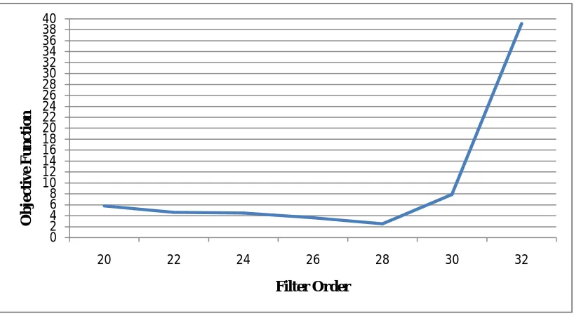
Initially, the PPO algorithm is run for 100 times and 200 iterations. The value of constant ‘a’ which represents maximum amplitude of effect of predator on prey is 0.0007× and constant ‘b’ for controlling the effect is 0.007/ . PPO has been implemented from 20 to 32 filter order. The variation of objective function with respect to filter orders has been depicted in Fig. 1.
Figure 1: Graph between Filter Order and achieved Objective Function
From the Fig. 1, it is clear that objective function keeps on decreasing from filter order 20 to 28. After filter order 28, the objective function rise steeply to very high value. Minimum objective function has been obtained at filter order 28 having value 2.506988.
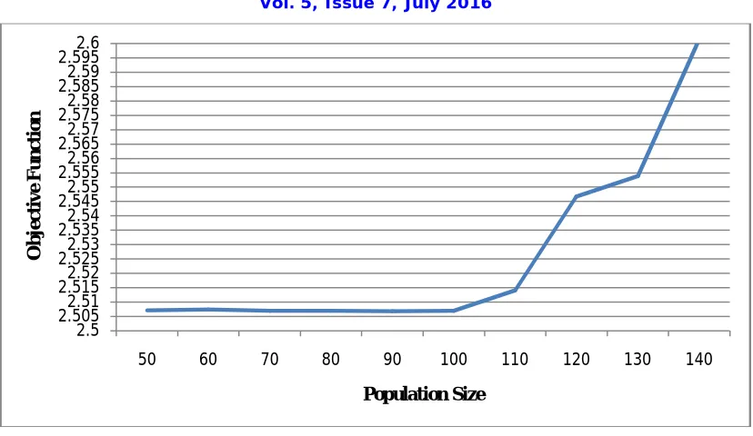
Further, on filter order 28, two control parameters i.e. population size and acceleration constants have been varied to attain minimal objective function. Firstly, population size has been varied from 50 to 140. The values of objective function at different populations have been drawn in the Fig. 2.
0 2 4 6 8 10 12 14 16 18 20 22 24 26 28 30 32 34 36 38 40
20 22 24 26 28 30 32
O
b
je
c
ti
v
e
F
u
n
c
ti
o
n
Figure 2: Graph of Objective Function versus Population Size at filter order 28
Fig. 2 shows that objective function keeps on decreasing from population size 50 to 90, and after that objective function raises abruptly. So, it observed that population size of 90 gives minimum objective value i.e. 2.506871. Secondly, another control parameter named as acceleration constants C1/C2 has been varied from 0.5 to 3.0 on population size 90.
Figure 3: Graph of Objective function versus Acceleration Constants (C1/C2) at filter order 28
It has been examined from Fig. 3 that the objective function gradually decreases for the value of C1/C2 from 0.5 to 1.5, and then it slightly decreases from 1.5 to 2. Further acceleration constant increases. Thus, it has been observed that the minimum value of objective function with population size 90 and acceleration constants C1/C2 equals to 2.0 is achieved as 2.506871.
Definitely, corollary is that optimal value of objective function has been attained on filter order 28, which demonstrates that total number of coefficients used in designing of the filter is 29. Low pass digital FIR filter designed using PPO algorithm, presents the results which are far away better than those obtained by using craziness based particle swarm optimization (CRPSO). Table 2 draws a comparison of objective function of PPO and CRPSO.
2.5 2.5052.51 2.5152.52 2.5252.53 2.5352.54 2.5452.55 2.5552.56 2.5652.57 2.5752.58 2.5852.59 2.5952.6
50 60 70 80 90 100 110 120 130 140
O
b
je
c
ti
v
e
F
u
n
c
ti
o
n
Population Size
2.506 2.507 2.508 2.509 2.51 2.511
0.5 1 1.5 2 2.5 3
O
b
je
c
ti
v
e
F
u
n
c
ti
o
n
Table 2: Comparison of Values of Objective Function of CRPSO and PPO
Sr. No. Technique Used Filter Order Objective Function
1 CRPSO
[10]
28 2.6910
2 PPO 28 2.506871
At filter order 28, design results for low pass digital FIR filter are depicted in Table 3 as given below:
Table 3: Design values for low pass digital FIR filter at filter order 28
Sr. No. Absolute magnitude error m1(x)
Squared magnitude error
) (
2 x
m
Pass-Band ripple error
) (x rp
Stop-Band ripple error rs(x)
1 1.329736 0.172664 0.049002 0.074532
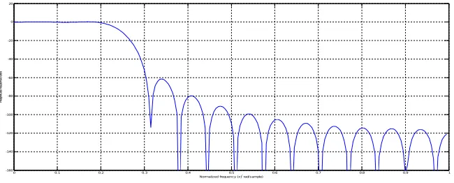
After obtaining the results, simulation has been carried out in MATLAB. The magnitude response has been plotted in Fig. 4.
Figure 4: Magnitude Response versus Normalized Frequency at filter order 28
The phase response from frequency range 0 to 0.3 has been plotted in Fig. 5 below.
Figure 5: Phase Response with respect to Normalized Frequency at filter order 28
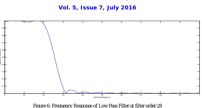
The frequency response of low pass digital FIR filter has been obtained from the coefficients as given in Fig. 6. The low pass filter passes the low frequencies while attenuating high frequencies.
0 0. 1 0. 2 0. 3 0.4 0.5 0.6 0.7 0.8 0.9 1
-160 -140 -120 -100 -80 -60 -40 -20 0 20
M
a
gn
it
ud
e
re
s
po
ns
e
(d
B
)
Normalized frequency (x rad/ sample)
0 0.1 0.2 0.3 0.4 0.5 0.6 0.7 0.8 0.9 1
-12 -10 -8 -6 -4 -2 0 2 4
P
h
as
e
r
es
p
o
n
s
e
(
d
e
g
re
e
s)
Figure 6: Frequency Response of Low Pass Filter at filter order 28
Table 4: Analytical calculation of Objective Function as well as Standard Deviation
Sr. No. Maximum value of Objective Function
Minimum value of Objective Function
Average value of Objective Function
Standard Deviation
1 2.533957 2.506871 2.507715 0.0191526
It is clear from the Table 4 that achieved standard deviation is less than 1, which reveals that the filter is robust in nature.
VI. CONCLUSION
This paper introduces predator-prey optimization method for the design of low pass digital FIR filter. The filter order has been varied from 20 to 32. Further two control parameters i.e. population size and acceleration constants C1 and C2 have been varied in order to obtain better results. On varying these variables, it has been concluded that optimal objective function has been obtained with population size 90 and value of acceleration constants C1 & C2 equals to 2.0. Best population has been selected using opposition based strategy. The achieved results using PPO have been compared with craziness based particle swarm optimization (CRPSO) for designing low pass digital FIR filter. From the corollary, it has been concluded that PPO has remarkable results in comparison to other techniques. The standard deviation conceded that designed filter is robust in nature because it has value less than one.
REFERENCES
[1] James Kennedy and Russell Eberhart, “Particle Swarm Optimization”, In Proceeding of IEEE International Conference on Neural Network, Perth Austraila, vol. 4,
no. 4, pp. 1942-1948, 1995.
[2] Shahryar Rahnamayan, Tizhoosh, and Salama, “Opposition-Based Differential Evolution”, IEEE Transactions on Evolutionary Computation, vol. 12, no. 1, pp.
64-79, 2008.
[3] Suman Kumar Sha, Rajib Kar, Durbadal Mandal and S. P. Ghoshal, “IIR Filter design with Craziness based Particle Swarm Optimization Technique”, International
Journal of Electrical, Computer, Energetic, Electronic and Communication Engineering, vol. 5, no. 12, pp. 1810-1817, 2011.
[4] Sonika Gupta and Aman Panghal, “Performance Analysis of FIR Filter Design by Using Rectangular, Hanning and Hamming Window Methods”, International
Journal of Advanced Research in Computer Science and Software Engineering, vol. 2, no. 6, pp. 273-277, 2012.
[5] Sangeeta Mondal, Dishari Chakraborty, Rajib Kar, Durbadal Mandal and Sakti Prasad Ghosal, “Novel Particle Swarm Optimization for High Pass FIR Filter
Design”, IEEE Symposium on Humanities, Science and Engineering Research, pp. 413-418, 2012.
[6] Ranjit Kaur, Manjeet Singh Patterh, J.S.Dhillon and Damanpreet Singh, “Heuristic Search Method for Digital IIR Filter Design”, WSEAS Transactions on Signal
Processing, vol. 8, no. 3, pp. 121-134, 2012.
[7] John Proakis and Dimitris Manolakis, “Digital Signal Processing: Principles, Algorithms and Applications”, Person Prentice Hall, Fourth Edition, 2013.
[8] Balraj Singh, J. S. Dhillon and Y. S. Brar, “Predator Prey Optimization method for the Design of IIR Method”, WSEAS Transactions on Signal Processing, vol. 9,
no. 2, pp. 51-63, 2013.
[9] Amrik Singh and Narwant Singh Grewal, “Review on FIR Filter Designing by Implementations of Different Optimization Algorithms”, International Journal of
Advanced Information Science and Technology, vol. 31, no. 31, pp. 171-175, 2014.
[10] Mohandeep Singh Sidhu and Darshan Singh Sidhu, “Design of Digital Low Pass FIR Filter Using Craziness Based Particle Swarm Optimization”, International
Journal of Advanced Research in Computer Science and Software Engineering, vol. 5, no. 6, pp. 667-674, 2015.
0 0.1 0.2 0.3 0.4 0.5 0.6 0.7 0.8 0.9 1
0 0.1 0.2 0.3 0.4 0.5 0.6 0.7 0.8 0.9 1
M
a
g
n
it
u
d
e
r
e
s
p
o
n
s
e